Circuit analysis for novices
This section is for those who want to analyse a circuit using a minimum of circuit theory!
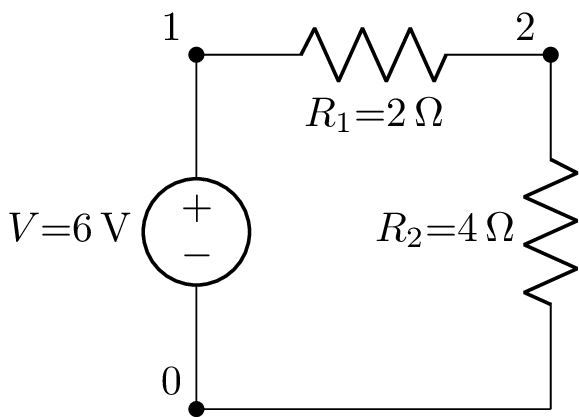
DC voltage divider
To analyse a voltage divider with Lcapy, it is necessary to create a netlist. For example:
>>> from lcapy import Circuit
>>> a = Circuit("""
... V 1 0 6; down=1.5
... R1 1 2 2; right=1.5
... R2 2 0_2 4; down
... W 0 0_2; right""")
>>> a.draw()
Each line of the netlist specifies a component. It has a name and nodes. The latter are usually numbers but can be alphanumeric. The first node is the more positive node. The options after a semicolon are optional but are useful for customising the schematic.
The voltage at each node (with respect to the ground node 0) can be found using:
>>> a[1].v
6
>>> a[2].v
4
The voltage across each component can be found using:
>>> a.V.v
6
>>> a.R1.v
2
>>> a.R2.v
4
Similarly, the current through each component can be found using:
>>> a.V.i
1
>>> a.R1.i
1
>>> a.R2.i
1
The units can be printed once this feature is enabled, for example:
>>> state.show_units=True
>>> state.abbreviate_units=True
>>> a.R1.i
1.A
>>> a.R1.v
2.V
>>> state.abbreviate_units=False
>>> a.R1.v
2.volt
AC voltage divider steady state response
An AC source can be created using the ac keyword when defining a voltage source. This has a default angular frequency \(\omega_0\).
>>> from lcapy import Circuit
>>> a = Circuit("""
... V 1 0 ac 6; down=1.5
... R 1 2 2; right=1.5
... C 2 0_2 4; down
... W 0 0_2; right""")
>>> a.draw()
Here, V 1 0 ac 6 is shorthand for V 1 0 {6 * cos(omega_0 * t)}.
The response to AC sources is gnarlier compared to DC sources:
>>> a.V.v
6⋅cos(ω₀⋅t)
>>> a.R.v
     2
384⋅ω₀ ⋅cos(ω₀⋅t)   48⋅ω₀⋅sin(ω₀⋅t)
───────────────── - ───────────────
         2                  2
    64⋅ω₀  + 1         64⋅ω₀  + 1

>>> a.R.v.simplify_sin_cos()
   _______________
  ╱        2
╲╱  2304⋅ω₀  + 36 ⋅cos(ω₀⋅t - atan(8⋅ω₀))
─────────────────────────────────────────
                     2
                64⋅ω₀  + 1
The interpretation is much easier using the concept of phasors.
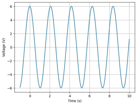
The voltage across R can be plotted, however, it needs a specific value for \(\omega_0\). For example:
>>> a.R.v.subs(omega0, 3).plot((-1, 10))
AC voltage divider step response
A change in amplitude (frequency or phase) of a signal produces a transient response. Here is a netlist with a voltage source that has a step change.
>>> from lcapy import Circuit
>>> a = Circuit("""
... V 1 0 step 6; down=1.5
... R 1 2 2; right=1.5
... C 2 0_2 4; down
... W 0 0_2; right""")
>>> a.draw()
Here, V 1 0 step 6 is shorthand for V 1 0 {6 * u(t)} where u(t) is Heaviside’s unit step.
The transient voltages are:
>>> a.V.v
6⋅u(t)
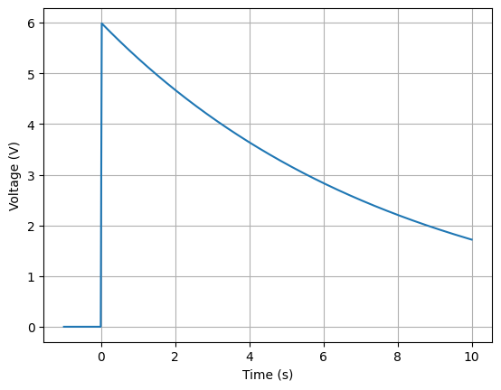
>>> a.R.v
-t
───
8
6⋅ℯ ⋅u(t)
>>> a.C.v
⎛ -t ⎞
⎜ ───⎟
⎜ 8 ⎟
3⋅⎝8 - 8⋅ℯ ⎠⋅u(t)
───────────────────
4
The voltage across R can be plotted using:
>>> a.R.v.plot((-1, 10))