Discrete-time signals
There are a number of domain variables for discrete-time signals:
n for discrete-time signals, for example, 3 * u(n - 2)
f for linear frequency from a DTFT
F for normalized linear frequency, F = f * dt
k for discrete-frequency spectra
omega for angular frequency from a DTFT, omega = 2 * pi * f
z for z-transforms, for example, Y(z)
Omega for normalized angular frequency from a DTFT, Omega = omega * dt
The n, k, and z variables share many of the attributes and methods of their continuous-time equivalents, t, f, and s, Expressions.
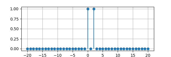
The discrete-time signal can be plotted using the plot() method. For example:
from lcapy import n, delta
from matplotlib.pyplot import savefig

x = delta(n) + delta(n - 2)
x.plot(figsize=(6, 2))

savefig('dt1-plot1.png')
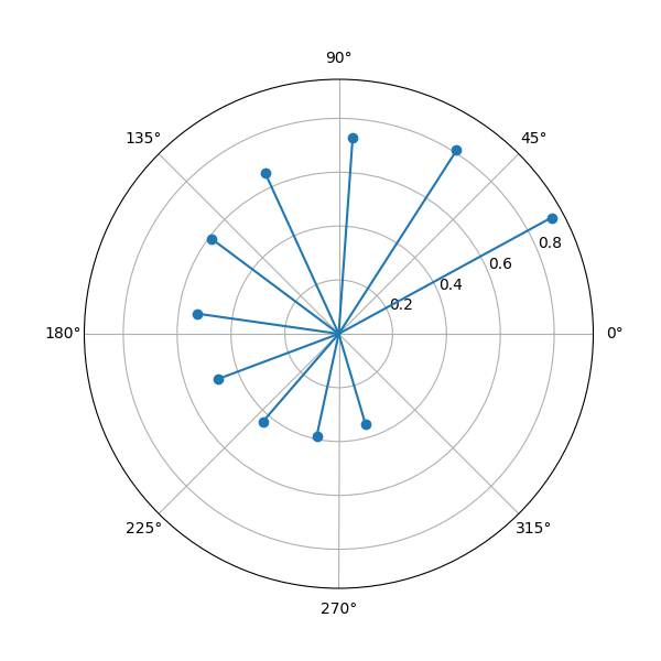
A complex discrete-time signal can be plotted in polar coordinates using the plot() method with the polar argument, for example:
from lcapy import j, n, exp
from matplotlib.pyplot import savefig

x = 0.9**n * exp(j * n * 0.5)
x.plot((1, 10), figsize=(6, 6), polar=True)

savefig('cdt1-plot1.png')
Functions
There are two special discrete time functions:
delta(n) or ui(n) or UnitImpulse(n): the discrete unit impulse. This is one when n=0 and zero otherwise.
u(n) or us(n) or UnitStep(n): the discrete unit step. This is one when n>=0 and zero otherwise.
Sequences
Generic sequences can be created using the seq function. For example:
>>> s = seq((1, 2, 3))
{_1, 2, 3}
Note, the underscore marks the element in the sequence where n = 0. By default, seq() creates a discrete-time domain sequence. The domain can be specified with the domain argument. This can be either n, k, or z. For example, a Z-domain sequence is created with:
>>> s = seq((1, 2, 3), domain=z)
{_1, 2, 3}
Here’s an example where the sequence is specified as a string:
>>> s = seq('1, _2, 3')
{1, _2, 3}
Sequences can also be generated from a discrete-time expression, for example:
>>> x = delta(n) + 2 * delta(n - 2)
>>> seq = x.seq((-5, 5))
>>> seq
{0, 0, 0, 0, 0, _1, 0, 2, 0, 0, 0}
Note, the underscore marks the origin; the element in the sequence where n = 0.
Sequences can have quantities, for example, a discrete-time voltage sequence is created with:
>>> v = voltage(seq((1, 2, 3), domain=n))
The extent of a sequence is given by the extent attribute.
>>> seq.extent
>>> 3
Each element in a sequence has a sequence index. The sequence indices are return as a list by the n attribute. For example:
>>> x = seq('1, _2, 3, 4')
>>> x.n
[-1, 0, 1, 2]
The origin of a sequence is given by the origin attribute. This indicates the element index where n = 0. For example:
>>> x = seq('1, _2, 3, 4')
>>> x.origin
1
>>> x = seq('1, 2, _3, 4')
>>> x.origin
2
The origin can be changed:
>>> x = seq('1, 2, _3, 4')
>>> x.origin = 1
>>> x
{1, _2, 3, 4}
Specific elements in the sequence can be accessed using call notation:
>>> x = seq('1, _2, 3, 4')
>>> x(0)
2
>>> x(1)
3
Specific elements can also be accessed using array notation. Note, the argument specifies the element sequence index, for example:
>>> x = seq('1, _2, 3, 4')
>>> x[0]
2
>>> x[1]
3
If you want the first element convert the sequence to a list or ndarray, for example:
>>> x = seq('1, _2, 3, 4')
>>> array(x)[0]
1
Sequences can be combined arithmetically, for example:
>>> seq((1, 2, 3)) + seq((4, 5)) - 1
{_4, 6, 2}

>>> seq((1, 2, 3)) * seq((4, 5)) * 2
{_8, 20, 0}
Note, the sequences are aligned using their sequence indices:
>>> seq((1, 2, 3)) + seq((4, 5), origin=-3)
{_1, 2, 3, 4, 5}
While this can be used to concatenate sequences, it is faster to use the append() method:
>>> seq((1, 2, 3)).append(seq((4, 5)))
{_1, 2, 3, 4, 5}
Multiple copies of a sequence can be appended using the repeat() method:
>>> seq((1, 2, 3)).repeat(2)
{_1, 2, 3, 1, 2, 3}
Sequences can be convolved with the convolve() method, for example:
>>> seq((1, 2, 3)).convolve(seq((1, 1))
{_1, 3, 5, 3}
Sequences can be evaluated and converted to a new sequence of floating point values using the evalf() method. This has an argument to specify the number of decimal places. For example:
>>> seq((pi, pi * 2))
{_π, 2⋅π}
>>> seq((pi, pi * 2)).evalf(3)
{_3.14, 6.28}
Sequences can be evaluated and converted to a NumPy array with the as_array() method:
>>> x = seq('1, _2, 3, 4')
>>> a = x.as_array()
>>> a
array([1., 2., 3., 4.])
Alternatively, the evaluate() method can be used to access and convert a single element or multiple elements. If the argument is a scalar, a real or complex Python scalar is returned. If the argument is iterable (tuple, list, ndarray), a NumPy real or complex ndarray is returned. Note, argument values outside the sequence return zero. Here is an example:
>>> x = seq('1, _2, 3, 4')
>>> x.evaluate(5)
0
>>> a = x.evaluate((1, 2))
>>> a
array([3., 4.])
Sequences can be converted to discrete-time domain or discrete-frequency domain expressions, for example:
>>> seq((1, 2)).expr
δ[n] + 2⋅δ[n - 2]
The discrete Fourier transform (DFT), inverse discrete Fourier transform (IDFT) z-transform (ZT), and inverse z-transform (IZT) can be performed using the DFT(), IDFT(), ZT(), and IZT() methods. In each case, a new sequence is returned. For example:
>>> seq((1, 2, 3, 4)).ZT()
⎧    2  3   4 ⎫
⎪_1, ─, ──, ──⎪
⎨    z   2   3⎬
⎪       z   z ⎪
⎩             ⎭

>>> seq((1, 2, 3, 4)).DFT()
{_10, -2 + 2⋅ⅉ, -2, -2 - 2⋅ⅉ}
Sequence operators
Lcapy overloads the leftshift operator and the rightshift operator to shift sequences. For example:
>>> a = seq((1, 2, 3))
>>> a >> 2
{_0, 0, 1, 2, 3}
>>> a << 2
{1, 2, _3}
Sequence attributes
expr convert to a discrete-time or discrete-frequency expression
extent the extent of the sequence
n the sequence indices
origin the element index for n = 0
vals the sequence values as a list
Sequence methods
These methods do not modify the sequence but return a new sequence, NumPy ndarray, or, Lcapy expression.
as_array() convert to NumPy ndarray
as_impulses() convert to a weighted sum of unit impulses expression
convolve() convolve with another sequence
delay() delay by an integer number of samples (the sequence is advanced if the argument is negative)
DFT() compute discrete Fourier transform as a sequence
DTFT() compute discrete-time Fourier transform
evalf() convert each element in sequence to a SymPy floating-point value with a specified number of digits
evaluate() evaluate sequence at specified indices and return as NumPy ndarray
IDFT() compute inverse discrete Fourier transform as a sequence
IZT() compute inverse z-transform as a sequence
lfilter() filter by DLTI filter
simplify() simplify each expression in sequence
prune() remove zeroes from the ends of the sequence
plot() plot sequence as a lollipop (stem) plot
zeroextend() add zeroes at either start or end so origin is included
zeropad() add zeroes to the end of the sequence
ZT() compute z-transform as a sequence
Sequence plotting
A sequence can be plotted using the plot() method. For example:
from lcapy import seq
from matplotlib.pyplot import savefig

x = seq((1, 2, 1, 0))
x.plot(figsize=(6, 2), unfilled=True)

savefig('seq1-plot.png')

Discrete-time (n-domain) expressions
Lcapy refers to Discrete-time expressions as n-domain expressions. They are of class DiscreteTimeDomainExpression and can be created explicitly using the n-domain variable n. For example:
>>> 2 * u(n) + delta(n - 1)
2⋅u[n] + δ[n - 1]
In this expression u(n) denotes the unit step and delta(n) denotes the unit impulse. Square brackets are used in printing to reduce confusion with the Heaviside function and Dirac delta.
Discrete-time expressions can be converted to sequences using the seq() method. For example:
>>> (delta(n) + 2 * delta(n - 1) + 3 * delta(n - 3)).seq()
{_1, 2, 0, 3}
The seq() method has an argument to specify the extent of the sequence. This is required if the sequences have infinite extent. For example:
>>> (2 * u(n) + delta(n - 1)).seq((-10, 10))
{_2, 3, 2, 2, 2, 2, 2, 2, 2, 2}
In this example the zero samples have been removed but the sequence has been truncated.
The z-transform of a discrete-time expression can be found with the ZT() method:
>>> (delta(n) + 2 * delta(n - 2)).ZT()
    2
1 + ──
     2
    z
A more compact notation is to pass z as an argument:
>>> (delta(n) + 2 * delta(n - 2))(z)
    2
1 + ──
     2
    z
The discrete-time Fourier transform (DTFT) of a discrete-time expression can be found with the DTFT() method:
>>> (delta(n) + 2 * delta(n - 2)).DTFT()
       -4⋅ⅉ⋅π⋅Δₜ⋅f
1 + 2⋅ℯ
A more compact notation is to pass f as an argument:
>>> (delta(n) + 2 * delta(n - 2))(f)
       -4⋅ⅉ⋅π⋅Δₜ⋅f
1 + 2⋅ℯ
The discrete Fourier transform (DFT) converts a discrete-time expression to a discrete-frequency expression. This is performed using the DFT() method or using a k argument. For example:
>>> (delta(n) + 2 * delta(n - 2))(k)
       -4⋅ⅉ⋅π⋅k
       ─────────
           N
1 + 2⋅ℯ
If N is known, it can be specified as an argument. For example:
>>> (delta(n) + 2 * delta(n - 2))(k, N=4)
       -ⅉ⋅π⋅k
1 + 2⋅ℯ
Evaluation of the DFT can be prevented by setting evaluate=False,
>>> (delta(n) + 2 * delta(n - 2))(k, N=4, evaluate=False)
  N
 ____
 ╲
  ╲                        -2⋅ⅉ⋅π⋅k⋅n
   ╲                       ───────────
   ╱                            N
  ╱   (δ[n] + 2⋅δ[n - 2])⋅ℯ
 ╱
 ‾‾‾‾
n = 0
Discrete-frequency (k-domain) expressions
Lcapy refers to discrete-frequency expressions as k-domain expressions. They are of class DiscreteFourierDomainExpression and can be created explicitly using the k-domain variable k. For example:
>>> 2 * u(k) + delta(k - 1)
2⋅u[k] + δ[k - 1]
Discrete-frequency expressions can be converted to sequences using the seq() method. For example:
>>> (delta(k) + 2 * delta(k - 1) + 3 * delta(k - 3)).seq()
{_1, 2, 0, 3}
Z-domain expressions
Z-domain expressions can be constructed using the z-domain variable z, for example:
>>> 1 + 1 / z
    1
1 + ─
    z
Alternatively, they can be generated using a z-transform of a discrete-time signal.
Z-domain expressions are objects of the ZDomainExpression class. They are functions of the complex variable z and are similar to LaplaceDomainExpression objects. The general form of a z-domain expression is a rational function so all the s-domain formatting methods are applicable (see Formatting methods).
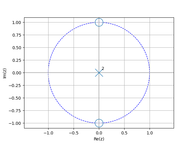
The poles and zeros of a z-domain expression can be plotted using the plot() method. For example:
from lcapy import delta
from lcapy.discretetime import n, z
from matplotlib.pyplot import savefig

x = delta(n) + delta(n - 2)
X = x(z)
X.plot()

savefig('dt1-pole-zero-plot1.png')
Transforms
Lcapy implements a number of transforms for converting between different domains. The explicit methods are:
DFT() Discrete Fourier transform
DTFT() Discrete-time Fourier transform
ZT() Z-transform
IDFT() Inverse discrete Fourier transform
IDTFT() Inverse discrete-time Fourier transform
IZT() Inverse z-transform
Z-transform (ZT)
Lcapy uses the unilateral z-transform, defined as:
The z-transform is performed explicitly with the ZT() method:
>>> x = delta(n) + 2 * delta(n - 2)
>>> x.ZT()
>>>      2
    1 + ──
         2
        z
It is also performed implicitly with z as an argument:
>>> x(z)
>>>     2
   1 + ──
        2
       z
Inverse z-transform (IZT)
The inverse unilateral z-transform is not unique and is only defined for \(n \ge 0\). For example:
>>> H = z / (z - 'a')
>>> H(n)
⎧ n
⎨a   for n ≥ 0
⎩
If the result is known to be causal, then use:
>>> H(n, causal=True)
 n
a ⋅u(n)
Discrete time Fourier transform (DTFT)
The DTFT converts an n-domain or z-domain expression into the f-domain (continuous Fourier domain). Note, unlike the Fourier transform, this is periodic with period \(1/\Delta t\). It is defined by
Note, there are other definitions, for example:
If \(x(n)\) is the impulse response of a causal and stable DLTI system, the DTFT can be found by substituting \(z = \exp(-2 \mathrm{j} \pi \Delta t f)\) into the z-transform of \(x(n)\).
Here is an example:
>>> sign(n).DTFT()
       2
────────────────
     -2⋅ⅉ⋅π⋅Δₜ⋅f
1 - ℯ
Alternatively, the transform can be invoked using f as an argument:
>>> sign(n)(f)
       2
────────────────
     -2⋅ⅉ⋅π⋅Δₜ⋅f
1 - ℯ
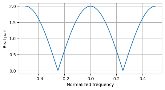
Here’s an example of plotting the DTFT:
from lcapy import delta
from lcapy.discretetime import n, dt
from matplotlib.pyplot import savefig

x = delta(n) + delta(n - 2)
abs(x.DTFT().subs(dt, 1)).plot(norm=True, figsize=(6, 3))

savefig('dt1-DTFT-plot1.png', bbox_inches='tight')
The DTFT can be confusing due to the number of definitions commonly used. Due to the periodicity it is common to define a normalized frequency \(F = f \Delta t\) and so
Here is an example:
>>> sign(n).DTFT(F)
      2
─────────────
     -2⋅ⅉ⋅π⋅F
1 - ℯ
Alternatively, the transform can be invoked using F as an argument:
>>> sign(n)(F)
      2
─────────────
     -2⋅ⅉ⋅π⋅F
1 - ℯ
Another option is to use normalized angular frequency \(\Omega = 2\pi f \Delta t\)
Here is an example:
>>> sign(n).DTFT(Omega)
      2
────────────────
     -2⋅ⅉ⋅π⋅Δₜ⋅f
1 - ℯ
Alternatively, the transform can be invoked using Omega as an argument:
>>> sign(n)(Omega)
      2
────────────────
     -2⋅ⅉ⋅π⋅Δₜ⋅f
1 - ℯ
A normalized discrete-time angular Fourier transform of x(n) can be plotted as follows:
>>> x.DTFT(Omega).plot()
This plots the normalized angular frequency between \(-\pi\) and \(\pi\).
The DTFT, \(X_{\frac{1}{\Delta t}}(f)\), is related to the Fourier transform, \(X(f)\), by
Note, some definitions do not include the scale factor \(1 / \Delta t\) since it assumed that \(x(n) = \Delta t x(n \Delta t)\). However, this introduces units confusion.
The DTFT is periodic in frequency with a period \(1 / \Delta t\) and provided the signal is not aliased, all the information about the signal can be obtained from any frequency range of interval \(1 / \Delta t\).
By default Lcapy returns an expression showing the infinite number of spectral images. For example,
>>> nexpr(1).DTFT()
   ∞
 ____
 ╲
  ╲
   ╲    ⎛    m ⎞
   ╱   δ⎜f - ──⎟
  ╱     ⎝    Δₜ⎠
 ╱
 ‾‾‾‾
m = -∞
────────────────
       Δₜ
All the images can be removed with the remove_images() method. For example:
>>> nexpr(1).DTFT().remove_images()
δ(f)
────
 Δₜ
Alternatively, the images argument can be used with the DTFT() method:
>>> nexpr(1).DTFT(images=0)
δ(f)
────
 Δₜ
The number of images can be specified with the m1 and m2 arguments to the remove_images() method. This is useful for plotting. For example,
>>> nexpr(1).DTFT(F).remove_images(-2, 2).doit()
δ(F) + δ(F - 2) + δ(F - 1) + δ(F + 1) + δ(F + 2)
Inverse discrete-time Fourier transform (IDTFT)
Like the DTFT, the IDFT has many commonly used definitions. In terms of linear frequency,
where \(x(n)\) denotes \(x(n \Delta t)\).
In terms of normalized linear frequency,
In terms of normalized angular frequency,
Discrete Fourier transform (DFT)
The DFT converts an n-domain expression to a k-domain expression. The definition used by Lcapy is:
Note, both \(x(n)\) and \(X(k)\) are assumed to periodic with period \(N\), i.e., \(x(n + m N) = x(n)\) for integer \(m\).
Inverse discrete Fourier transform (IDFT)
The IDFT converts a k-domain expression to an n-domain expression. The definition used by Lcapy is:
Again, both \(x(n)\) and \(X(k)\) are assumed to periodic with period \(N\), i.e., \(x(n + m N) = x(n)\) for integer \(m\).
Bilinear transform
The bilinear transform can be used to approximate an s-domain expression with a z-domain expression using \(s \approx \frac{2}{\Delta t} \frac{1 - z^{-1}}{1 + z^{-1}}\) (see Discrete-time approximation for other methods). This is performed by the bilinear_transform() method of s-domain objects, for example:
>>> H = s / (s - 'a')
>>> Hz = H.bilinear_transform().simplify()
>>> Hz
      2⋅(1 - z)
──────────────────────
Δₜ⋅a⋅(z + 1) - 2⋅z + 2
The related method inverse_bilinear_transform() converts an s-domain expression to the z-domain using \(z \approx (1 + 0.5 \Delta t s) / (1 - 0.5 \Delta t s)\).
Here’s an example of the bilinear transform applied for an RC low-pass filter.
>>> from lcapy import Circuit, s, t
>>> net = Circuit("""
R 1 2; right
W 0 0_2; right
C 2 0_2; down
W 2 3; right=0.5
W 0_2 0_3; right=0.5""")
This has a transfer function:
>>> H = net.transfer(1, 0, 3, 0)
>>> H
      1
─────────────
    ⎛     1 ⎞
C⋅R⋅⎜s + ───⎟
    ⎝    C⋅R⎠
and an impulse response:
>>> H(t)
 -t
 ───
 C⋅R
e   ⋅u(t)
─────────
   C⋅R
Using the bilinear transform, the discrete-time transfer function is
>>> H.bilinear_transform().canonical()
          Δₜ⋅(z + 1)
──────────────────────────────
⎛    -2⋅C⋅R + Δₜ⎞
⎜z + ───────────⎟⋅(2⋅C⋅R + Δₜ)
⎝     2⋅C⋅R + Δₜ⎠
with a discrete-time impulse response
>>> from lcapy.discretetime import n
>>> H.bilinear_transform()(n).simplify()
   ⎛                  n                         ⎞
   ⎜      ⎛2⋅C⋅R - Δₜ⎞                          ⎟
Δₜ⋅⎜4⋅C⋅R⋅⎜──────────⎟ ⋅u(n) - (2⋅C⋅R + Δₜ)⋅δ[n]⎟
   ⎝      ⎝2⋅C⋅R + Δₜ⎠                          ⎠
─────────────────────────────────────────────────
            (2⋅C⋅R - Δₜ)⋅(2⋅C⋅R + Δₜ)