Expressions¶

Lcapy expressions are similar to SymPy expressions except they have a specific domain depending on the predefined domain variables t, s, f, F omega (w), Omega (W), jf, and jomega (jw). They have associated quantities, domains, and units.

Introduction¶

Lcapy expressions are comprised of numbers, pre-defined constant symbols, domain variables, user-defined symbols, and functions.

Numbers¶

Lcapy approximates real numbers as rationals. This ensures expected simplifications of expressions. However, some floating-point numbers produce unwieldy rationals (see Floating point values) and so it is best to avoid floating-point numbers. For example, use:

>>> expr('2 / 3')

or

>>> expr(one * 2 / 3)

rather than

>>> expr(2 / 3)

The floating-point approximation can be found using fval attribute for a Python float or cval for a Python complex number:

>>> expr(2 / 3).fval
0.166666666666667

>>> expr(2 / 3).cval
(0.16666666666666666+0j)

Rational numbers in Lcapy expressions can be converted to SymPy floating-point numbers using the evalf() method, with a specified number of decimal places. For example:

>>> expr('1 / 3 + a').evalf(5)
a + 0.33333

If you prefer floating-point numbers use the ratfloat() method. For example:

>>> expr('0.1 * a')
a
──
10
>>> expr('0.1 * a').ratfloat()
0.1⋅a

The companion method floatrat() converts floating-point numbers to rational numbers.

Constants¶

pi 3.141592653589793…
j \(\sqrt{-1}\)
oo infinity
zoo complex infinity
one 1

Domain variables¶

Lcapy has eight predefined domain variables for continuous time signals:

t – time domain
f – Fourier (frequency) domain
F – normalized Fourier (frequency) domain (\(F = f \Delta t\))
s – Laplace (complex frequency) domain
omega (or w) – angular Fourier domain (\(\omega = 2 \pi f\))
Omega (or W) – normalized angular Fourier domain (\(\Omega = \omega \Delta t\))
jf – frequency response domain
jomega (or jw) – angular frequency response domain

A time-domain expression is produced using the t variable, for example:

>>> e = exp(-3 * t) * u(t)

Similarly, a Laplace-domain expression is produced using the s variable, for example:

>>> V = s / (s**2 + 2 * s + 3)

There are an additional three domain variables for discrete-time signals (see Discrete-time signals):

n – discrete-time domain
k – discrete-frequency domain
z – z-domain

For example:

>>> V = delta(n) + 2 * delta(n - 1) + 3 * delta(n - 3)

All Lcapy expressions have a domain (Laplace, Fourier, etc.) and a quantity (voltage, current, undefined) etc. For example:

>>> V = voltage(5 * t)
>>> V.domain
'time'
>>> V.quantity
'voltage'

A voltage expression can also be created by multiplying an expression by a voltage unit. For example:

>>> V = 5 * t * volts
>>> V.domain
'time'
>>> V.quantity
'voltage'

This applies to the units: volts, amperes, ohms, siemens, and watts. Note, this is experimental and may be deprecated since the resultant units might be too confusing.

User-defined symbols¶

Symbols can also be created with Lcapy’s symbol function. For example:

>>> tau = symbol('tau', real=True)
>>> N = symbol('N', even=True)

They are also implicitly created from strings using the expr() function. For example:

>>> v = expr('exp(-t / tau) * u(t)')

or

>>> v = voltage('exp(-t / tau) * u(t)')

Notes:

Lcapy maintains a registry of symbols, created both explicitly and implicitly. This includes special symbols such as j and pi, domain symbols such as s and t (associated with the domain variables), and user-defined symbols.
By default, symbols are assumed to be positive, unless explicitly specified not to be. For example:
```
>>> a = symbol('a', negative=True)
```
Symbols created with the symbol() or symbols() function are printed verbatim. For example:
```
>>> xest = symbol('\hat{x}')
\hat{x}
```
Symbols created with expr() are printed in a canonical form. For example, R1 is printed as R_1, even though it is stored as R1.
Some symbols are previously defined by SymPy. These can be redefined using symbol or symbols but not with expr unless the override argument is True. For example:
```
>>> mypi = symbol('pi')
```
or
```
>>> e = expr('pi / 4', override=True)
```
In both cases, the special number symbol pi becomes an arbitrary symbol.
Domain symbols (t, f, etc.) can only be redefined with force=True. Caveat emptor! This can cause confusion. For example:
```
>>> n = symbol('n', force=True, real=True)
```

Mathematical functions¶

Lcapy has the following built-in functions: sin, cos, tan, cot, asin, acos, atan, atan2, acot, sinh, cosh, tanh, asinh, acosh, atanh, gcd, exp, sqrt, log, log10, sign, conjugate, rect, dtrect, sinc, sincn, sincu, tri, trap, Heaviside, H, u, DiracDelta, delta, unitimpulse, unitstep, Piecewise, Derivative, Integral, integrate, diff, Min, and Max among others.

Other SymPy functions can be converted to Lcapy functions using the Function class, for example:

>>> import sympy as sym
>>> gamma = Function(sym.gamma)
>>> gamma(4)
6

For additional details on some of these functions see Special functions.

Domains¶

Lcapy uses a variety of domains to represent signals. This helps with circuit analysis since time-domain convolutions simplify to multiplications in the Fourier, Laplace, and phasor domains. Lcapy uses the following transform domains for circuit analysis:

Constant domain for DC signals
Phasor domain for AC signals
Laplace domain (s-domain) for transient signals
Fourier domain (and angular Fourier domain) for noise signals

The domain of an expression is usually determined from the pre-defined domain variables (see Domain variables). For example:

>>> Z = impedance(3 * s)
>>> Z.domain
'laplace'

However, this is not possible for constants. One approach is to use:

>>> Z = impedance(0 * s + 5)
>>> Z.domain
'laplace'

Alternatively, there are a number of functions for setting the domain:

cexpr() set constant domain
fexpr() set Fourier domain
Fexpr() set normalized Fourier domain
omegaexpr() set angular Fourier domain
Omegaexpr() set normalized angular Fourier domain
sexpr() set Laplace domain
texpr() set time domain
phasor() set phasor domain

For example:

>>> Z = impedance(sexpr(5))
>>> Z.domain
'laplace'

There are restrictions on how expressions can be combined. In general, both expressions must be of the same domain and have compatible quantities. For example, you cannot do:

>>> 5 * t + 4 * s
ValueError: Cannot determine TimeDomainExpression(5*t) + LaplaceDomainExpression(4*s) since the domains are incompatible

Expressions can be transformed to different domains, see Domain transformation.

Domain attributes¶

is_undefined_domain
is_constant_domain
is_time_domain
is_laplace_domain
is_fourier_domain
is_angular_fourier_domain
is_norm_fourier_domain
is_norm_angular_fourier_domain
is_frequency_response_domain
is_angular_frequency_response_domain
is_phasor_domain
is_phasor_ratio_domain
is_discrete_time_domain
is_discrete_fourier_domain
is_Z_domain
is_transform_domain

Domain classes¶

Lcapy has many expression classes, one for each combination of domain (time, Fourier, Laplace, etc) and expression type (voltage, current, impedance, admittance, transfer function). For example, to represent Laplace domain entities there are the following classes:

LaplaceDomainExpression is a generic s-domain expression.

LaplaceDomainVoltage is a s-domain voltage.

LaplaceDomainCurrent is a s-domain current.

LaplaceDomainTransferFunction is a s-domain transfer function.

LaplaceDomainAdmittance is a s-domain admittance.

LaplaceDomainImpedance is a s-domain impedance.

These classes should not be explicitly used. Instead use the factory functions expr, voltage, current, transfer, admittance, and impedance.

Phasors¶

Phasors represent signals of the form \(v(t) = A \cos(\omega t + \phi)\) as a complex amplitude \(X = A \exp(\mathrm{j} \phi)\) where \(A\) is the amplitude, \(\phi\) is the phase, and the angular frequency, \(\omega\), is implied. The signal corresponding to the phasor \(A \exp(\mathrm{j} \phi)\) is found from:

\[x(t) = \mathrm{Re}\left\{ A \exp(\mathrm{j} \phi) \exp(\mathrm{j} \omega t)\right\}\]

Thus, the signal \(v(t) = A \sin(\omega t)\) has a phase \(\phi=-\pi/2\).

Phasors can be created in Lcapy with the phasor() factory function:

>>> P = phasor(2)
>>> P.time()
2⋅cos(ω⋅t)

>>> P = phasor(-2 * j)
>>> P.time()
2⋅sin(ω⋅t)

The default angular frequency is omega but this can be specified:

>>> phasor(-j, omega=1)
sin(t)

Phasors can also be inferred from an AC signal:

>>> P = phasor(2 * sin(3 * t))
>>> P
-2⋅ⅉ
>>> P.omega
3

Phasor voltages and currents can be created using the voltage() and current() functions. For example:

>>> V = voltage(phasor(1))
>>> V.quantity
'voltage'

They can also be created from an AC time-domain signal using the as_phasor() method. For example:

>>> v = voltage(2 * sin(7 * t))
>>> V = v.as_phasor()
>>> V
-2⋅ⅉ

Like all Lcapy expressions, the magnitude and phase of the phasor can be found from the magnitude and phase attributes. For example:

>>> V = voltage(phasor(2 * sin(7 * t)))
>>> V.magnitude
2
>>> V.phase
-π
───
 2

The root-mean-square value of the phasor is found with the rms() method. For example:

>>> V = voltage(phasor(2))
>>> V.rms()
√2

Phasors can be plotted on a polar diagram using the plot() method, for example:

>>> I = current(phasor(1 + j))
>>> I.plot()

Phasor ratios¶

The ratio of two phasors is a phasor ratio; it is not a phasor. For example:

>>> V = voltage(phasor(4))
>>> I = current(phasor(2))
>>> Z = V / I
>>> Z.domain
phasor ratio
>>> Z.omega
ω

Noise signals¶

Lcapy can represent wide-sense stationary, zero-mean, Gaussian random processes. They are represented in terms of their one-sided, amplitude spectral density (ASD); this is the square root of the power spectral density (PSD), assuming a one ohm load.

With the wide-sense stationary assumption, random process can be described by their power spectral (or amplitude spectral) density or by their time-invariant autocorrelation function.

Lcapy assumes each noise source is independent and assigns a unique noise identifier (nid) to each noise expression produced from a noise source. A scaled noise expression shares the noise identifier since the noise is perfectly correlated.

Consider the sum of two noise processes:

\[Z(t) = X(t) + Y(t).\]

With the wide-sense stationarity and independence assumptions, the resulting-power spectral density is given by

\[S_Z(f) = S_X(f) + S_Y(f),\]

and the amplitude spectral density is

\[\mathcal{A}_Z(f) = \sqrt{\mathcal{A}_X^2(f) + \mathcal{A}_Y^2(f)}.\]

Furthermore, the resultant autocorrelation is

\[R_Z(\tau) = R_X(\tau) + R_Y(\tau).\]

Noise signals can be created using the noisevoltage() and noisecurrent() methods. For example, a white-noise signal can be created using:

>>> X = noisevoltage(3)
>>> X.units
'V/sqrt(Hz)'
>>> X.domain
'fourier noise'
>>> X.nid
1

When another white-noise signal is created, it is is assigned a different noise identifier since the noise signals are assumed to be independent:

>>> Y = noisevoltage(4)
>>> Y.nid
2

Since the noise signals are independent and wide-sense stationary, the ASD of the result is found from the square root of the sum of the squared ASDs:

>>> Z = X + Y
>>> Z
5

Care must be taken when manipulating noise signals. For example, consider:

>>> X + Y - X
√34
>>> X + Y - Y
√41

The error arises since it is assumed that X + Y is independent of X which is not the case. A work-around is to create a VoltageSuperposition object until someone comes up with a better idea. This stores each independent noise component separately (as used by Lcapy when performing circuit analysis). For example:

>>> from lcapy.superpositionvoltage import SuperpositionVoltage
>>> X = noisevoltage(3)
>>> Y = noisevoltage(4)
>>> Z = SuperpositionVoltage(X) + SuperpositionVoltage(Y)
{n1: 3, n2: 4}
>>> Z = SuperpositionVoltage(X) + SuperpositionVoltage(Y) - SuperpositionVoltage(X)
{n2: 4}

Quantities¶

Each expression has a quantity (voltage, current, undefined, etc.). When combining expressions, the quantity of the result is determined for the most common combination of electrical quantities. For example:

>>> V = current(1 / s) * impedance(2)
>>> V.quantity
'voltage'

However, there are restrictions on how expressions can be combined. For example, you cannot do:

>>> voltage(3) + current(4)
ValueError: Cannot determine ConstantVoltage(3) + ConstantCurrent(4) since the units of the result are unsupported.
As a workaround use x.as_expr() + y.as_expr()

There are a number of methods for changing the quantity of an expression:

as_expr() removes the quantity (it is set to ‘undefined’)
as_voltage() converts to voltage
as_current() converts to current
as_impedance() converts to impedance
as_admittance() converts to admittance
as_transfer() converts to transfer function
as_power() converts to power

There are similar functions for setting the quantity of an expression:

expr() removes the quantity
voltage() converts to voltage
current() converts to current
impedance() converts to impedance
admittance() converts to admittance
transfer() converts to transfer function

An Lcapy quantity is not a strict quantity but a collection of related quantities, For example, both voltage (with units V) and voltage spectral density (with units V/Hz) are considered voltage quantities. However, they have different units.

Quantity attributes¶

Expressions have the following attributes to identify the quantity:

is_voltage
is_current
is_impedance
is_admittance
is_transfer
is_immitance
is_voltagesquared
is_currentsquared
is_impedancesquared
is_admittancesquared
is_power

Immittances¶

Immittances (impedances and admittances) are a frequency domain generalization of resistance and conductance. In Lcapy they are represented using the Impedance and Admittance classes for each of the domains. The appropriate class is created using the impedance and admittance factory functions. For example:

>>> Z1 = impedance(5 * s)
>>> Z2 = impedance(5 * j * omega)
>>> Z3 = admittance(s * 'C')

The impedance can be converted to a specific domain using a domain variable as an argument. For example:

>>> Z1(omega)
5⋅ⅉ⋅ω
>>> Z2(s)
5⋅s
>>> Z1(f)
10⋅ⅉ⋅π⋅f

The time-domain representation of the immittance is the inverse Laplace transform of the s-domain immittance, for example:

>>> impedance(1 / s)(t)
Heaviside(t)
>>> impedance(1)(t)
δ(t)
>>> impedance(s)(t)
 (1)
δ   (t)

Here \(\delta^{(1)}(t)\) denotes the time-derivative of the Dirac delta, \(\delta(t)\).

An Admittance or Impedance object can be created with the Y or Z attribute of a Oneport component, for example:

>>> C(3).Z
-ⅉ
───
3⋅ω

>>> C(3).Z(s)
 1
───
3⋅s
>>> C(3).Y(s)
3⋅s

Netlist components have similar attributes. For example:

>>> from lcapy import Circuit
>>> a = Circuit("""
... C 1 2""")
>>> a.C.Z
 1
───
C⋅s

Immittance attributes¶

B susceptance
G conductance
R resistance
X reactance
Y admittance
Z impedance
is_lossy has a non zero resistance component

Impedance is related to resistance and reactance by

\(Z = R + \mathrm{j} X\)

Admittance is related to conductance and susceptance by

\(Y = G + \mathrm{j} B\)

Since admittance is the reciprocal of impedance,

\(Y = \frac{1}{Z} = \frac{R}{R^2 + X^2} - \mathrm{j} \frac{X}{R^2 + X^2}\)

Thus

\(G = \frac{R}{R^2 + X^2}\)

and

\(B = \frac{-X}{R^2 + X^2}\)

Note, at DC, when \(X = 0\), then \(G = 1 / R\) and is infinite for \(R= 0\). However, if Z is purely imaginary, i.e, \(R = 0\) then \(G = 0\), not infinity as might be expected.

Immittance methods¶

oneport() returns a Oneport object corresponding to the immittance. This may be a R, C, L, G, Y, or Z object.

Voltages and currents¶

Voltages and currents are created with the voltage() and current() factory functions. For example:

>>> v = voltage(5 * u(t))
>>> I = current(5 * s)

The domain is inferred from the domain variable in the expression (see Domains).

The results from circuit analysis are represented by a superposition of different domains.

Voltage and current superpositions¶

Superpositions of voltages and/or current are represented using the SuperpositionVoltage and SuperpositionCurrent classes. These classes have similar behaviour; they represent an arbitrary voltage or current signal as a superposition of DC, AC (phasor), transient, and noise signals.

For example, the following expression is a superposition of a DC component, an AC component, and a transient component:

>>> V1 = SuperpositionVoltage('1 + 2 * cos(2 * pi * 3 * t) + 3 * u(t)')
>>> V1
⎧          3        ⎫
⎨dc: 1, s: ─, 6⋅π: 2⎬
⎩          s        ⎭

This shows that there is 1 V DC component, a transient component with a Laplace transform \(3 / s\), and an AC component (phasor) with amplitude 2 V and angular frequency \(6 \pi\) rad/s.

Pure DC components are not shown as a superposition. For example:

>>> V2 = SuperpositionVoltage(42)
>>> V2
42

Similarly, pure transient components are not shown as a superposition if they depend on s. For example:

>>> V3 = SuperpositionVoltage(3 * u(t))
>>> V3
3
─
s

However, consider the following:

>>> V4 = SuperpositionVoltage(4 * DiracDelta(t))
>>> V4
{s: 4}

This is not shown as 4 to avoid confusion with a 4 V DC component. Maybe it should be written \(0 s + 4\)?

A pure AC component (phasor) has magnitude, phase, and omega attributes. The latter is the angular frequency. For example:

>>> V5 = SuperpositionVoltage(3 * sin(7 * t) + 4 * cos(7 * t))
>>> V5
{7: 4 - 3⋅ⅉ}
>>> V5.magnitude
5

If the signal is a superposition of AC signals, each phasor can be extracted using its angular frequency as the index. For example:

>>> V6 = SuperpositionVoltage(3 * sin(7 * t) + 2 * cos(14 * t))
>>> V6[7]
-3⋅ⅉ
>>> V6[14]
2

The signal can be converted to another domain using a domain variable as an argument:

V1(t) returns the time domain expression
V1(f) returns the Fourier domain expression with linear frequency
V1(s) returns the Laplace domain expression
V1(omega)`or `V1(w) returns the angular Fourier domain expression
V1(jomega) or V1(jw) returns the angular frequency domain expression

Here are some examples:

>>> V1(t)
2⋅cos(6⋅π⋅t) + 3⋅u(t) + 1
>>> V1(s)
  ⎛ 2       2⎞
6⋅⎝s  + 24⋅π ⎠
──────────────
  ⎛ 2       2⎞
s⋅⎝s  + 36⋅π ⎠
>>> V1(jomega)
     ⎛   2       2⎞
-6⋅ⅉ⋅⎝- ω  + 24⋅π ⎠
────────────────────
    ⎛   2       2⎞
  ω⋅⎝- ω  + 36⋅π ⎠

Voltage and current attributes¶

dc returns the DC component
ac returns a dictionary of the AC components, keyed by the frequency
transient returns the time-domain transient component
is_dc returns True if a pure DC signal
is_ac returns True if a pure AC signal
is_transient returns True if a pure transient signal
has_dc returns True if has a DC signal
has_ac returns True if has an AC signal
has_transient returns True if has a transient signal
domain returns the domain as a string
quantity returns the quantity (voltage or current) as a string
is_voltage returns True if a voltage expression
is_current returns True if a current expression

In addition, there are domain attributes, such as is_time_domain, is_laplace_domain, etc. (see Domain attributes).

Voltage and current methods¶

oneport() returns a Oneport object corresponding to the immittance. This may be a V or I object.

Units¶

Expressions have an attribute units that reflect the quantity and domain. For example:

>>> voltage(7).units
V
>>> voltage(7 * f).units
V
──
Hz
>>> voltage(7 / s).units
V
──
Hz
>>> voltage(7 * s).units
V
──
Hz
>>> s.units
rad
───
 s

The units are a SymPy Expression and thus can be formatted as a string, LaTeX, etc. They can be automatically printed, for example:

>>> state.show_units = True
>>> voltage(7)
7⋅V

Abbreviated units are employed by default, however, this can be disabled. For example:

>>> state.show_units = True
>>> state.abbreviate_units = False
>>> voltage(7)
7⋅volt

By default, units are printed in the form they are created. However, they can be printed in a simplified canonical form:

>>> state.show_units = True
>>> current(7) * impedance(2)
14⋅A⋅ohm
>>> state.canonical_units = True
>>> current(7) * impedance(2)
14⋅V

Alternatively, the units can be simplified using the simplify_units() method:

>>> state.show_units = True
>>> V = current(7) * impedance(2)
>>> V
14⋅A⋅ohm
>>> V.simplify_units()
14⋅V

The units are chosen as a function of quantity and domain when an Lcapy expression is created and are modified by multiplications, divisions, and transformations, such as a Fourier transform. Here are the default values:

+-------------------+-----+-------+--------+------+--------+-----+--------+-----+-----+-----+-----------+
| Quantity/Domain   | dc  | t     | s      | f    | omega  | jf  | jomega | n   | k   | z   | noise f   |
+-------------------+-----+-------+--------+------+--------+--------+-----+-----+-----+-----+-----------+
| Voltage           | V   | V     | V/Hz   | V/Hz | V/Hz   | V   | V      | V   | V   | V   | V/sqrt(Hz)|
+-------------------+-----+-------+--------+------+--------+-----+--------+-----+-----+-----+-----------+
| Current           | A   | A     | A/Hz   | A/Hz | A/Hz   | A   | A      | A   | A   | A   | A/sqrt(Hz)|
+-------------------+-----+-------+--------+------+--------+-----+--------+-----+-----+-----+-----------+
| Impedance         | ohm | ohm/s | ohm    | ohm  | ohm    | ohm | ohm    | ohm | ohm | ohm |           |
+-------------------+-----+-------+--------+------+--------+-----+--------+-----+-----+-----+-----------+
| Admittance        | S   | S/s   | S      | S    | S      | S   | S      | S   | S   | S   |           |
+-------------------+-----+-------+--------+------+--------+-----+--------+-----+-----+-----+-----------+
| Transfer function | 1   | 1/s   | 1      | 1    | 1      | 1   | 1      | 1   | 1   | 1   |           |
+-------------------+-----+-------+--------+------+--------+-----+--------+-----+-----+-----+-----------+

Note, the transfer functions are assumed to be voltage or current ratios in the Laplace and Fourier domains. Voltage and current ratios are represented by impedances and admittances.

Unit determination goes awry when some mathematical functions are used. For example:

>>> log(voltage(7)).units
V

Unit attributes¶

Expressions have the following attributes for units:

units returns the units as a SymPy expression
canonical_units returns the units as a SymPy expression in canonical form (volt * ampere is converted to watts, 1 / s is converted to Hz, etc.)
expr_with_units returns a SymPy expression multiplied by the units

Containers¶

Lists¶

Lcapy uses its own list type ExprList that wraps each element as an Lcapy Expr object. For example,

>>> a = expr([t, t**2, '3 * t'])
>>> a
⎡    2     ⎤
⎣t, t , 3⋅t⎦

An ExprList can be converted to a list suitable for sympy using the sympy attribute:

>>> a.sympy
⎡    2     ⎤
⎣t, t , 3⋅t⎦
ExprList objects have many similar printing methods to Expr objects such as pprint() and latex(). Other methods include:
subs(symbol, value) substitutes symbol with value.

subs(defs) substitutes symbols where defs is a dictionary of values keyed by symbol name
solve() solves a system of equations, for example,
>>> v = expr('v(t)')
>>> vR = expr('vR(t)')
>>> vL = expr('vL(t)')
>>> i = expr('i(t)')
>>> R = symbol('R')
>>> L = symbol('L')
>>> system = expr([Eq(v, vR + vL), Eq(vR, i * R), Eq(vL, Derivative(i, t) * L)])
>>> unknowns = expr((vR, vL, i))
>>> # Solve in Laplace domain
>>> solutions = system(s).solve(unknowns(s))
>>> solutions
⎧        V(s)           L⋅s⋅V(s)           R⋅V(s)⎫
⎨I(s): ───────, V_L(s): ────────, V_R(s): ───────⎬
⎩      L⋅s + R          L⋅s + R           L⋅s + R⎭
fval() evaluates each expression in the list and return a list of Python float values

cval() evaluates each expression in the list and return a list of Python complex values

Tuples¶

Lcapy uses its own tuple type ExprTuple that wraps each element as an Lcapy Expr object. For example,

>>> a = expr((t, t**2, '3 * t'))
>>> a
⎛    2     ⎞
⎝t, t , 3⋅t⎠

ExprTuple objects have the same methods and attributes as ExprList objects.

Dicts¶

Lcapy uses its own dict type ExprDict that wraps each element and key as an Lcapy Expr object. For example,

>>> expr({1:t, 't':2 * t, 4 * t:2 * t})
{t: 2⋅t, 1: t, 4⋅t: 2⋅t}

ExprDict objects share the printing methods of ExprTuple and ExprList objects.

Matrices¶

Matrix objects are created with the Matrix class. Currently, there are different flavours of Matrix class for the different domains, for example, LaplaceDomainMatrix and TimeDomainMatrix. These are likely to be replaced with a generic Matrix class in the future. Here’s an example of usage:

>>> Matrix(((1, t), (3, '4')))
⎡1  t⎤
⎢    ⎥
⎣3  4⎦

Note, currently, the quantity associated with each matrix element is lost. The Matrix class subclasses the SymPy Matrix class and thus all the SymPy Matrix methods are supported, such as inv() to invert a matrix and det() to calculate the determinant.

Vectors¶

Vector objects are created with the Vector class. These are a subclass of the Matrix class.

Signals and transfer functions¶

Lcapy expressions represent signals or the behaviour of a system.

Signals are voltage or current quantities (or their products such as instantaneous power). The signals are either driving functions (excitation functions) or responses (such as the voltage across a component or the current through a component). Signals can be constant (DC), AC, transient, or a combination of AC, DC, and transient. A causal signal is zero for \(t < 0\).

The behaviour of a system is described in a transform domain (Laplace, Fourier, or phasor) by a transfer function. This is the ratio of two transformed signals, for example, \(H(s) = V_2(s) / V_1(s)\). Impedances, \(Z(s) = V(s) / I(s)\), and admittances, \(Y(s) = I(s) / V(s)\), are a special kind of transfer function.

The time domain representation of a transfer function, \(H(s)\), is called the impulse response, \(h(t)\). For a causal system, \(h(t) = 0\) for \(t < 0\).

Rational functions¶

Linear time-invariant systems have transfer functions that are rational functions; the ratio of two polynomials:

\[H(s) = \frac{N(s)}{D(s)},\]

The numerator can be found using the N attribute and denominator can be found using the D attribute. For example:

>>> Z = impedance((5 * s) / (s**2 + 5 * s + 6))
       5⋅s
 ────────────
  2
 s  + 5⋅s + 6
 >>> Z.N
 5⋅s
 >>> Z.D
  2
 s  + 5⋅s + 6

Responses¶

Usually, s-domain responses are rational functions but if there is a time delay there is an additional exponential factor. So, in general, Lcapy tries to interpret responses as

\[V(s) = \sum_{i} \frac{N_i(s)}{D(s)} \exp(-s \tau_i),\]

where \(\tau_i\) are time delays. This representation is returned by the as_sum() method. Note, these expressions cannot be represented in Factored (ZPK) form. The D attribute returns \(D(s)\) and the N attribute returns

\[N(s) = \sum_{i} N_i(s) \exp(-s \tau_i).\]

Expression attributes¶

All Lcapy expressions have the following attributes (see Rational functions and Responses for definitions of numerator and denominator):

abs returns absolute value
angle returns phase angle (radians)
cartesian returns expression in form real + j * imag
conj returns complex conjugate (equivalent to conjugate() method)
cval returns complex floating-point number (as Python complex) if expression can be evaluated (see also val, fval, and evalf())
dB returns magnitude in decibels: 20 * log10(magnitude)
D returns denominator
Ddegree returns degree of denominator
denominator returns denominator
degree returns degree (order) of rational function (maximum of numerator and denominator degrees)
domain returns a string identifying the domain (laplace, fourier, etc.)
domain_label returns string describing domain of expression
expr returns the underlying SymPy expression
fval returns floating-point number (as Python float) if expression can be evaluated (see also val, cval, and evalf())
imag returns imaginary part
is_ac returns True if AC signal
is_causal returns True if signal is causal, i.e, is 0 for \(t < 0\)
is_conditional returns True if expression is conditional, e.g., \(\exp(-t)\;\; t \ge 0\)
is_constant returns True if expression is constant (it must have no free symbols, compare with is_unchanging), e.g., 3 is constant but 3 * x is not
is_dc returns True if DC signal
is_marginally_stable returns True if the Laplace transform of the expression has all its poles in the LH plane or on the boundary
is_number returns True if expression is a number
is_rational_function returns True if expression is a rational function
is_realizable returns True if the Laplace transform of the expression is 0 in the limit as \(s\) tends to infinity. This is equivalent to the Laplace transform of the expression being strictly proper (the degree of the numerator being greater than the degree of the numerator). Note, by this definition cos(t) is considered realizable
is_stable returns True if the Laplace transform of the expression has all its poles in the LH plane
is_strictly_proper returns True if degree of denominator greater than degree of numerator
is_unchanging returns True if expression does not have a domain variable (compare with is_constant), e.g., 3 * x is unchanging but 3 * t is not
label returns string describing expression to use as a plot label
magnitude returns absolute value
N returns numerator
Ndegree returns degree of numerator
numerator returns numerator
phase returns phase (radians)
phase_degrees returns phase (degrees)
polar returns expression in form mag * exp(j * phase)
quantity returns a string identifying the quantity (voltage, current, undefined, etc.)
real returns real part
real_imag returns expression in form real + j * imag
sign returns sign of expression
symbols returns dictionary of symbols used in the expression keyed by their names
val returns floating-point number (as Lcapy expression) if expression can be evaluated (see also fval, cval, and evalf())
var returns the underlying SymPy symbol representing the domain

In addition, each expression has domain, quantity, and unit attributes, see Domain attributes, Quantity attributes, and Unit attributes.

Expression methods¶

Poles and zeros¶

coeffs() returns list of coefficients if the expression is a polynomial; the highest powers come first. If the expression is a rational function use .N.coeffs or .D.coeffs for the numerator or denominator coefficients.
normcoeffs() returns list of coefficients if the expression is a polynomial; the highest powers come first. The coefficients are normalized so the highest order coefficient is 1. If the expression is a rational function use .N.coeffs or .D.coeffs for the numerator or denominator coefficients.
poles(aslist) returns poles of expression as a dictionary or a list if the aslist argument is True. Note, this does not always find all the poles (see roots()).
roots(aslist) returns roots of expression as a dictionary or a list if the aslist argument is True. Note, this does not always find all the roots, for example, if the degree is five or more (https://en.wikipedia.org/wiki/Abel%E2%80%93Ruffini_theorem). In this case, if the polynomial coefficients are constants, the roots are calculated numerically.
zeros(aslist) returns zeros of expression as a dictionary or a list if the aslist argument is True. Note, this does not always find all the zeros (see roots()).

Transforms¶

FT() Fourier transform, see Fourier transforms
IFT() Inverse Fourier transform, see Inverse Fourier transforms
LT() Laplace transform, see Laplace transforms
ILT() Inverse Laplace transform, see Inverse Laplace transforms

Miscellaneous¶

as_sum() rewrites expression as a sum of terms where the denominator of each term has a common polynomial expression (see Responses).
convolve(x) convolves expressions (see Convolution).

The result is an unevaluated integral. It can be evaluated using the doit() method.

Note, this method not simplify the convolution integral if one of the functions contains a Dirac delta. This can be done using the simplify_dirac_delta() method.
differentiate() differentiates expression.
discretize(method=’bilinear’) converts the expression to a discrete-time approximation, see Discrete-time approximation.
divide_top_and_bottom(expr) divides numerator and denominator by expr.

dlti_filter(method=’bilinear’) creates a DLTI filter (see Discrete-time linear time invariant filters) by approximating the discrete-time impulse response (see Discrete-time approximation). For example,

>>> H = transfer(1 / (s + 'a'))
>>> fil = H.dlti_filter()
>>> fil.a
⎛   Δₜ⋅a - 2⎞
⎜1, ────────⎟
⎝   Δₜ⋅a + 2⎠
>>> fil.b
⎛   Δₜ        Δₜ   ⎞
⎜────────, ────────⎟
⎝Δₜ⋅a + 2  Δₜ⋅a + 2⎠
>>> fil.difference_equation()
       Δₜ⋅x(n)    Δₜ⋅x(n - 1)   (Δₜ⋅a - 2)⋅y(n - 1)
y(n) = ──────── + ─────────── - ───────────────────
       Δₜ⋅a + 2     Δₜ⋅a + 2          Δₜ⋅a + 2

evalf(n) returns floating-point number to n decimal places (as Lcapy expression) if expression can be evaluated (see also val, fval, and cval attributes)
evaluate(arg) returns floating-point number (Python float or complex type) if expression can be evaluated. If passed a tuple, list, or NumPy array, an array of NumPy float or complex types is returned. For example:
```
>>> (t**2 + 4).evaluate(1)
5
>>> (t**2 + 4).evaluate((1, 2))
array([5., 8.])
```
initial_value() returns result at \(t = 0\).
integrate(arg, **kwargs) integrates expression. For example:
```
>>> exp(-3 * t).integrate((t, 0, oo))
1 / 3
```
factor_const() factors expression into constant part and the rest.
final_value() returns result at \(t = \infty\).
force_causal() removes the piecewise condition and multiplies expression by Heaviside unit step (only for time-domain expression), for example:
```
>>> (1/s)(t)
1  for t ≥ 0
>>> (1/s)(t).force_causal()
u(t)
```
limit() computes a limit.
multiply_top_and_bottom(expr) multiplies numerator and denominator by expr.
nsolve(x0, **kwargs) returns numerical solution with x0 as the starting point close to the solution. See sympy.solvers.solvers.nsolve for details.

parameterize() parameterizes first, second, and third order rational functions into common forms. For example:

>>> H, defs = (1 / (5 * s**2 + 10 * s + 20)).parameterize()
>>> H
         K
───────────────────
  2               2
ω₀  + 2⋅ω₀⋅s⋅ζ + s
>>> defs
{K: 1/5, omega_0: 2, zeta: 1/2}
H, defs = (1 / (5 * s**2 + 10 * s + 20)).parameterize(zeta=False)
>>> H
           K
───────────────────────
  2    2              2
ω₁  + s  + 2⋅s⋅σ₁ + σ₁
>>> defs
{K: 1/5, omega_1: √3, sigma_1: 1}

parameterize_ZPK() parameterizes rational functions into zero-pole-gain (ZPK) form. For example:

>>> H, defs = (1 / (5 * s**2 + 10 * s + 20)).parameterize_ZPK()
>>> H
           1
K⋅───────────────────
  (-p₁ + s)⋅(-p₂ + s)
>>> defs
{K: 1/5, p1: -1 - √3⋅ⅉ, p2: -1 + √3⋅ⅉ}

post_initial_value() returns result at \(t = 0^{+}\) (only for time-domain and Laplace-domain expression).
pre_initial_value() returns result at \(t = 0^{-}\) (only for time-domain expression).
rationalize_denominator() multiplies numerator and denominator by complex conjugate of denominator to ensure the new denominator is purely real.
remove_condition() removes the piecewise condition (only for time-domain expression), for example:
```
>>> (1/s)(t)
1  for t ≥ 0
>>> (1/s)(t).remove_condition()
1
```
replace(query, value) replaces query with value.
response(xvector, tvector, method=’bilinear’) determines the discrete time-domain response given an input vector xvector at the instants specified by tvector.
rewrite(args, hints) rewrites expression in terms of the args. For example, exp(j*a*t).rewrite(cos) gives ⅉ⋅sin(4⋅t) + cos(4⋅t). Similarly, cos(2 * t).rewrite(exp) will expand the cosine as two complex exponentials.
solve(symbols, flags) returns list of solutions. For example:
```
>>> (s**2 - 4).solve()
[-2, 2]
```
term_const() splits expression into constant part and the rest.

Convolution¶

The convolution() method has two different forms:

>>> expr('i(t)').convolve(expr('z(t)'))
∞
⌠
⎮  i(t - τ)⋅z(τ) dτ
⌡
-∞
>>> expr('i(t)').convolve(expr('z(t)'), commutate=True)
∞
⌠
⎮  i(τ)⋅z(t - τ) dτ
⌡
-∞

The infinite limits of the convolution integral are constrained if either of the functions is known to be causal. For example:

>>> expr('i(t)').convolve(expr('z(t)', causal=True))
∞
⌠
⎮  i(t - τ)⋅z(τ) dτ
⌡
0
>>> expr('i(t)', causal=True).convolve(expr('z(t)'))
t
⌠
⎮  i(t - τ)⋅z(τ) dτ
⌡
-∞
>>> expr('i(t)', causal=True).convolve(expr('z(t)', causal=True))
t
⌠
⎮  i(t - τ)⋅z(τ) dτ
⌡
0

The convolve() method does not simplify the convolution integral, for example:

>>> expr('i(t)').convolve(expr('u(t)'))
∞
⌠
⎮  i(t - τ)⋅u(τ) dτ
⌡
0
>>> expr('i(t)').convolve(expr('u(t)')).simplify()
∞
⌠
⎮  i(t - τ) dτ
⌡
0

Formatting methods¶

Lcapy expressions can be displayed in many forms. For example, consider the s-domain rational-function:

>>> H = 5 * (s**2 + 1) / (s**2 + 5*s + 4)

Canonical form¶

The canonical form has a unity coefficient for the highest power in the denominator. It is sometimes called polynomial form.

>>> H.canonical()
  ⎛   2    ⎞
  ⎝5⋅s  + 5⎠
────────────
 2
s  + 5⋅s + 4

There is a variation of the canonical form which has a unity coefficient for the highest power in the denominator and with constants factored in the numerator. It is sometimes called gain-polynomial form.

>>> H.canonical(factor_const=True)
   ⎛ 2    ⎞
 5⋅⎝s  + 1⎠
────────────
 2
s  + 5⋅s + 4

Expanded canonical form¶

The expanded canonical form expresses the rational function into the sum of rational functions where the numerator of each term contains a unique monomial.

>>> H.expandcanonical()
       2
    5⋅s             5
──────────── + ────────────
 2              2
s  + 5⋅s + 4   s  + 5⋅s + 4

General form¶

The general form of a rational function is shown as the ratio of two polynomials. Unlike the canonical form, the coefficient for the highest power in the denominator may not be unity.

>>> H.general()
     2
  5⋅s  + 5
────────────
 2
s  + 5⋅s + 4

Factored (ZPK) form¶

The factored form shows both the numerator and denominator polynomials factored. It is an alias for ZPK (zero-pole-gain) form.

>>> H.factored()
5⋅(s - ⅉ)⋅(s + ⅉ)
─────────────────
 (s + 1)⋅(s + 4)

Complex conjugate pairs are combined when the pairs argument is True to create a product of biquad sections.

>>> H.factored(pairs=True)
       2
    5⋅s  + 5
───────────────
(s + 1)⋅(s + 4)

Partial fraction form¶

The partial fraction form has terms that are strictly proper.

>>> H.partfrac()
        85          10
5 - ───────── + ─────────
    3⋅(s + 4)   3⋅(s + 1)

The recippartfrac() method generates a partial fraction expansion using the reciprocal of the variable:

>>> H.recipartfrac()
5       10          85
─ - ───────── + ──────────
4     ⎛    1⎞      ⎛1   1⎞
    3⋅⎜1 + ─⎟   48⋅⎜─ + ─⎟
      ⎝    s⎠      ⎝4   s⎠

The partfrac() and recippartfrac() methods have a pairs argument. If this is True, a sum of biquad sections is created. For example:

>>> H = 5 / (s * (s**2 + 1))
>>> H.partfrac()
      5           5       5
- ───────── - ───────── + ─
  2⋅(s + ⅉ)   2⋅(s - ⅉ)   s
>>> H.partfrac(pairs=True)
      5⋅s     5
   - ────── + ─
      2       s
     s  + 1

Standard form¶

The standard form expresses the rational function as the sum of a polynomial and a strictly proper rational function.

>>> H.standard()
   25⋅s + 15
- ──────────── + 5
   2
  s  + 5⋅s + 4

Time constant form¶

The time constant form factors the rational function into gain-time-constant form.

>>> H.timeconst()
5⋅(-ⅉ⋅s + 1)⋅(ⅉ⋅s + 1)
──────────────────────
    ⎛s    ⎞
  4⋅⎜─ + 1⎟⋅(s + 1)
    ⎝4    ⎠

Printing methods¶

pprint() pretty print an expression
latex() convert an expression to LaTeX string representation
pretty() convert an expression to a string with a prettified form
plot() plot the expression, provided there are no free symbols (see Plotting)

There are a number of global printing options, controlled by attributes of the state object.

state.show_units (default False) prints the units after an expression
state.canonical_units (default True) converts units to canonical form, e.g., V / A is shown as ohms.
state.printing.abbreviate_units (default True) prints V rather than volts
state.printing.order (default None) controls the order that symbols in an expression are printed. When order =None, SymPy orders the printed arguments and produces output like -p + s. When order=’none’, SymPy does not order the printed arguments. However, when creating an expression, SymPy sorts the argument order for commutative operators (such as add) and does not honour how the expression was created.

SymPy methods¶

If Lcapy does not have a method defined but the underlying SymPy expression does, the SymPy method is used. For example:

diff()
expand()

Utility functions¶

symbol() creates a symbol
expr() creates an expression. This can also create lists, tuples, and dictionaries of expressions.

Note, SymPy does not allow symbol names that are Python keywords. For example, expr(‘is(t)’) fails. A workaround is to use an underscore in the name, for example, expr(‘i_s(t)’).

Domain transformation¶

Expressions can be transformed to a different domain (see Domains and Domain transformation), for example. This can be done with an explicit method, for example, the Fourier transform can be determined with:

>>> cos(4 * pi * t).FT(f)
 δ(f - 2)   δ(f + 2)
──────── + ────────
   2          2

>>>  x.FT(omega)
π⋅(δ(ω - 4⋅π) + δ(ω + 4⋅π))

Alternatively, the call notation can be used to choose the new domain:

- `V(t)` returns the time domain transformation

V(f) returns the Fourier domain transformation
V(F) returns the normalized Fourier domain transformation
V(s) returns the Laplace domain (s-domain) transformation
V(omega) returns the angular Fourier domain transformation
V(Omega) returns the normalized angular Fourier domain transformation
V(jf) returns the frequency response domain transformation
V(jomega) or V(jw) returns the angular frequency response domain transformation
V(n) returns the discrete-time domain transformation (by default the bilinear-transform is used)
V(k) returns the discrete-frequency domain transformation (by default the bilinear-transform is used)
V(z) returns the Z-domain transformation (by default the bilinear-transform is used)

For example:

>>> from lcapy import *
>>> V1 = voltage('3 * exp(-2 * t)')
>>> V1(t)
   -2⋅t
3⋅e
>>> V1(s)
  3
─────
s + 2

Transformation and substitution use a similar syntax V(arg). If arg is a domain variable t, f, s, omega, w, jf, jomega, jw, n, k, or z or is an expression of a domain variable, transformation is performed, otherwise substitution is performed. This behaviour can be explicitly controlled using the subs() and transform() methods, for example:

>>> from lcapy import *
>>> V1 = voltage('3 * exp(-2 * t)')
>>> V1.transform(s)
  3
─────
s + 2
>>> V1.transform(t)
   -2⋅t
3⋅e
>>> V1.subs(2)
   -4
3⋅e
>>> V1.subs(2).evaluate()
0.054946916666202536

Here’s another example:

>>> Hf = 1e6 / (j * f / 10 + 1)
1000000
───────
ⅉ⋅f
─── + 1
 10
>>> Hs = Hf.subs(f, s / (j * 2 * pi)).canonical()
20000000⋅π
──────────
 s + 20⋅π

Frequency response and Fourier domains (jomega or omega)¶

The transformation V(omega) produces a result in the angular Fourier domain, however, the transformation V(jomega) produces a result in the angular frequency response domain. In most cases, V(omega) produces the same result as V(jomega) but not always. Here’s an example where the two domains produce the same expression:

>>> Y = admittance(s)
>>> Y(omega)
ⅉ⋅ω
>>> Y(jomega)
ⅉ⋅ω

While they look the same, they have different domains:

>>> Y(omega).domain
'angular fourier'
>>> Y(jomega).domain
'angular frequency response'

Here’s an example, showing a subtle difference between the angular Fourier and angular frequency response domains for the impedance of a 1 F capacitor:

>>> Z = impedance(1 / s)
>>> Z(omega)
  ⎛ ω ⎞
 δ⎜───⎟
  ⎝2⋅π⎠   ⅉ
 ────── - ─
   2      ω
>>> Z(jomega)
 -ⅉ
 ───
  ω

In this case, substitution of s with jomega is not valid to obtain the Fourier transform. This is because the poles of Z are not in the RH plane (they are on the imaginary axis and thus the system is marginally stable) and thus the evaluation of Z(s) at s = jomega is outside the region of convergence of the Laplace transform.

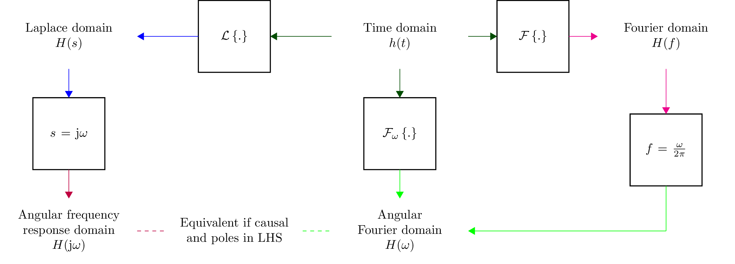
The following diagram demonstrates transformations between the domains. Note, the unilateral Laplace transform denoted by \(\mathcal{L}\{.\}\) is not reversible without some prior information (the region of convergence). In general, the result is only known for \(t\ge 0\) since the result for \(t < 0\) is not unique. The Fourier transform, denoted by \(\mathcal{F}\{.\},\) and the angular Fourier transform, denoted by \(\mathcal{F}_{\omega}\{.\}\), are reversible. If \(h(t)\) is an AC signal, it is possible to go between the time and phasor domains. If \(H(s)\) represents the transfer function of a causal system with all its poles in the LH plane, then it is possible to go between the Laplace and angular Fourier domains via the phasor ratio domain. Note, the capitalized expressions denote a transform domain and are not equivalent.

Fourier transforms¶

Lcapy uses the following definition of the forward Fourier transform:

\[V(f) = \mathcal{F}\{v(t)\} = \int_{-\infty}^{\infty} v(t) \exp(-\mathrm{j} 2\pi f t) \mathrm{d}t\]

The Fourier transform can be performed with the explicit FT() method:

>>> f0 = symbol('f0')
>>> cos(2 * pi * f0 * t).FT()
  δ(f - f₀)   δ(f + f₀)
 ───────── + ─────────
     2           2

Alternatively it can be performed using call notation:

>>> f0 = symbol('f0')
>>> cos(2 * pi * f0 * t)(f)
  δ(f - f₀)   δ(f + f₀)
 ───────── + ─────────
     2           2

>>> (rect(t) * cos(2 * pi * f0 * t))(f)
 sinc(f - 1)   sinc(f + 1)
 ─────────── + ───────────
      2             2

Inverse Fourier transforms¶

Lcapy uses the following definition of the inverse Fourier transform: .. math:

v(t) = \mathcal{F}^{-1}\{V(f)\} = \int_{-\infty}^{\infty} V(f) \exp(\mathrm{j} 2\pi f t) \mathrm{d}f

The inverse Fourier transform can be performed with the explicit IFT() method:

>>> DiracDelta(f - 4).IFT()
  8⋅ⅉ⋅π⋅t
 ℯ

Alternatively it can be performed using call notation:

>>> DiracDelta(f - 4)(t)
  8⋅ⅉ⋅π⋅t
 ℯ

Angular Fourier transforms¶

Lcapy uses the following definition of the forward angular Fourier transform:

\[V(\omega) = \mathcal{F}_{\omega}\{v(t)\} = \int_{-\infty}^{\infty} v(t) \exp(-\mathrm{j} \omega t) \mathrm{d}t\]

and the following definition of the inverse angular Fourier transform:

\[v(t) = \mathcal{F}_{\omega}^{-1}\{V(\omega)\} = \frac{1}{2\pi}\int_{-\infty}^{\infty} V(\omega) \exp(\mathrm{j} \omega t) \mathrm{d}\omega\]

The angular Fourier transform can be performed with the explicit FT() method with omega or w as an argument:

>>> f0 = symbol('f0')
>>> cos(2 * pi * f0 * t).FT(omega)
 π⋅(δ(2⋅π⋅f₀ - ω) + δ(2⋅π⋅f₀ + ω))

Alternatively:

>>> rect(t)(w)
     ⎛ ω ⎞
 sinc⎜───⎟
     ⎝2⋅π⎠

Laplace transforms¶

There are three variants of the unilateral Laplace transform used in circuit theory texts. Lcapy uses the \(\mathcal{L}_{-}\) form where:

\[\mathcal{L}_{-}\{v(t)\} = \int_{0^{-}}^{\infty} v(t) \exp(-s t) \mathrm{d}t\]

SymPy uses the \(\mathcal{L}\) form where:

\[\mathcal{L}\{v(t)\} = \int_{0}^{\infty} v(t) \exp(-s t) \mathrm{d}t\]

The third form is \(\mathcal{L}_{+}\) where:

\[\mathcal{L}_{+}\{v(t)\} = \int_{0^{+}}^{\infty} v(t) \exp(-s t) \mathrm{d}t\]

The choice of lower limit is most important for the Dirac delta distribution (and its derivatives): \(\mathcal{L}_{-}\{\delta(t)\} = 1\) but \(\mathcal{L}\{\delta(t)\} = 0.5\) and \(\mathcal{L}_{+}\{\delta(t)\} = 0\).

The \(\mathcal{L}_{-}\) form is advocated for circuit analysis in the paper Initial conditions, generalized functions, and the Laplace transform: Troubles at the origin by K. Lundberg, H. Miller, R. Haynes, and D. Trumper in IEEE Control Systems Magazine, Vol 27, No 1, pp. 22–35, 2007, http://dedekind.mit.edu/~hrm/papers/lmt.pdf

The time-derivative rule for the \(\mathcal{L}_{-}\) Laplace transform is:

\[\mathcal{L}_{-}\{v'(t)\} = s V(s) - v(0^{-}),\]

where \(v(0^{-})\) is the pre-initial value of \(v\).

Laplace transforms are performed with the LT() method:

>>> f0 = symbol('f0')
>>> cos(2 * pi * f0 * t).LT()
       s
 ─────────────
    2   2    2
 4⋅π ⋅f₀  + s

Alternatively, using call notation:

>>> f0 = symbol('f0')
>>> cos(2 * pi * f0 * t)(s)
       s
 ─────────────
    2   2    2
 4⋅π ⋅f₀  + s

Derivatives of generic functions produce results with initial conditions. For example:

>>> Derivative('v(t)')(s)
s⋅V(s) - v(0)

>>> Derivative('v(t)', t, 2)(s)
 2                 ⎛d       ⎞│
s ⋅V(s) - s⋅v(0) - ⎜──(v(t))⎟│
                   ⎝dt      ⎠│t=0

If the initial conditions are zero:

>>> Derivative('v(t)')(s, zero_initial_conditions=True)
s⋅V(s)

Alternatively, the initial conditions can be removed by the zero_initial_conditions() method:

>>> Derivative('v(t)')(s).zero_initial_conditions()
s⋅V(s)

Versions of Lcapy prior to 1.5.3 assumed zero initial conditions. This behaviour can be restored using:

>>> from lcapy import state
>>> state.zero_initial_conditions = True

Inverse Laplace transforms¶

Inverse Laplace transforms are performed with the ILT() method:

>>> (1 / (s + 4)).ILT()
  -4⋅t
 ℯ      for t ≥ 0

Alternatively, using call notation:

>>> (1 / (s + 4))(t)
  -4⋅t
 ℯ      for t ≥ 0

If the result is known to be causal, use the causal argument:

>>> (1 / (s + 4))(t, causal=True)
  -4⋅t
 ℯ     u(t)

Alternatively, the condition can be removed by the remove_condition() method:

>>> (1 / (s + 4))(t).remove_condition()
  -4⋅t
 ℯ

or the expression can be forced to be causal using the force_causal() method:

>>> (1 / (s + 4))(t).force_causal()
  -4⋅t
 ℯ     u(t)

Inverse Laplace transforms of a generic function multiplied by a power of s produces a result with initial conditions:

>>> (s * 'V(s)')(t)
            d
v(0)⋅δ(t) + ──(v(t))
            dt

If the initial conditions are known to be zero use:

>>> (s * 'V(s)')(t, zero_initial_conditions=True)
d
──(v(t))
dt

Alternatively, the initial conditions can be removed by the zero_initial_conditions() method:

>>> (s * 'V(s)')(t).zero_initial_conditions()
d
──(v(t))
dt

Versions of Lcapy prior to 1.5.3 assumed zero initial conditions. This behaviour can be restored using:

>>> from lcapy import state
>>> state.zero_initial_conditions = True

With second order systems, the form of the result can be modified using the damping argument. This can be ‘under’, ‘over’, or ‘critical’, for example:

>>> expr('1/(s**2 + a*s + b)')(t, damping='under', causal=True)
⎛         ⎛               ____________⎞        ⎛               ____________⎞⎞
⎜         ⎜  a           ╱    2       ⎟        ⎜  a           ╱    2       ⎟⎟
⎜       t⋅⎜- ─ - 0.5⋅ⅉ⋅╲╱  - a  + 4⋅b ⎟      t⋅⎜- ─ + 0.5⋅ⅉ⋅╲╱  - a  + 4⋅b  ⎟⎟
⎜         ⎝  2                        ⎠        ⎝  2                        ⎠⎟
⎜1.0⋅ⅉ⋅ℯ                                  ⅉ⋅ℯ                                ⎟
⎜────────────────────────────────────── - ──────────────────────────────────⎟⋅ u(t)
⎜              ____________                           ____________          ⎟
⎜             ╱    2                                 ╱    2                 ⎟
⎝           ╲╱  - a  + 4⋅b                         ╲╱  - a  + 4⋅b           ⎠

Compare this with:

>>> expr('1/(s**2 + a*s + b)')(t, damping='over', causal=True)
⎛     ⎛         __________⎞      ⎛         __________⎞⎞
⎜     ⎜        ╱  2       ⎟      ⎜        ╱  2       ⎟⎟
⎜     ⎜  a   ╲╱  a  - 4⋅b ⎟      ⎜  a   ╲╱  a  - 4⋅b ⎟⎟
⎜   t⋅⎜- ─ - ─────────────⎟    t⋅⎜- ─ + ─────────────⎟⎟
⎜     ⎝  2         2      ⎠      ⎝  2         2      ⎠⎟
⎜  ℯ                          ℯ                       ⎟
⎜- ──────────────────────── + ────────────────────────⎟⋅u(t)
⎜          __________                 __________      ⎟
⎜         ╱  2                       ╱  2             ⎟
⎝       ╲╱  a  - 4⋅b               ╲╱  a  - 4⋅b       ⎠

Expression manipulation¶

Substitution¶

Substitution replaces sub-expressions with new sub-expressions in an expression. It is most commonly used to replace the underlying variable with a constant, for example:

>>> a = 3 * s
>>> b = a.subs(2)
>>> b
6

Since the replacement expression is a constant, the substitution can also be performed using the call notation:

>>> b = a(2)
>>> b
6

With two arguments, subs() replaces a symbol with an expression. For example,

>>> a = expr('a * t + b')
>>> a.subs('a', 2)
b + 2⋅t

With one iterable argument of new/old pairs, subs() iterates over each pair. For example:

>>> a = expr('a * t + b')
>>> a.subs((('a', 4), ('b', 2))
4⋅t + 2

The substitution method can also have a dictionary argument, keyed by symbol name, to replace symbols in an expression with constants. For example:

>>> a = expr('a * t + b')
>>> a.subs({'a': 4, 'b': 2})
4⋅t + 2

If you know what you are doing you can coerce the domain of the result with the domain argument, for example:

>>> H.subs(f, w / (2 * pi)).subs(jw, s, domain=s)

Evaluation¶

Evaluation is similar to substitution but requires all symbols in an expression to be substituted with values. The result is a numerical answer, for example:

>>> a = expr('t**2 + 2 * t + 1')
>>> a.evaluate(0)
1.0

The argument to evaluate can be a scalar, a tuple, a list, or a NumPy array. For example:

>>> a = expr('t**2 + 2 * t + 1')
>>> tv = np.linspace(0, 1, 5)
>>> a.evaluate(tv)
array([1.    , 1.5625, 2.25  , 3.0625, 4.    ])

If the argument is a scalar the returned result is a Python float or complex type; otherwise it is a NumPy array. The evaluation method is useful for plotting results, (see Plotting).

Simplification¶

Lcapy has the following simplification methods:

doit() evaluates a summation or integral, for example:
```
>>> Sum(n, (n, 0, 4)).doit()
10
```
simplify() augments the SymPy simplification function by also simplifying expressions containing Dirac deltas and Heaviside steps.

simplify_conjugates() combines complex conjugate terms, for example:

>>> (exp(j * 3) + exp(-j * 3) + 1).simplify_conjugates()
2⋅cos(3) + 1

simplify_dirac_delta() simplifies Dirac deltas.
simplify_heaviside() simplifies Heaviside unit steps, for example:
```
>>> (u(t) * u(t)).simplify_heaviside()
u(t)
```
simplify_factors() simplifies each factor separately.
simplify_rect() simplifies expressions with rectangle functions, for example:
```
>>> (rect(t) * rect(t)).simplify_rect()
rect(t)
```
simplify_sin_cos() rewrites sums of sines and cosines in terms of a single phase-shifted-sine or cosine, for example:
```
>>> (3 * sin(omega0 * t) + 4 * cos(omega0 * t)).simplify_sin_cos()
5⋅cos(ω₀⋅t - atan(3/4))
```
simplify_terms() simplifies each term separately.
simplify_units() simplifies the units of an expression, for example, V/A becomes ohms.
simplify_unit_impulse() simplifies unit impulses.
expand_hyperbolic_trig converts sinh, cosh, tanh into sum of exponentials. For example:
```
>>> (sinh(s) + cosh(s)).expand_hyperbolic_trig()
   s
2⋅ℯ
```
expand_functions converts functions into simpler forms. For example:
```
>>> rect(t).expand_functions()
-u(t - 1/2) + u(t + 1/2)
```

Approximation¶

Lcapy has the following approximation methods:

approximate_dominant(defs, threshold) approximates expression: using ball-park numerical values for the symbols to decide which terms in a sum dominate the sum. For example,

>>> expr('1/(A * B + A * A + C)').approximate_dominant('A':100,'B':1,'C':20}, 0.005)
      1
 ────────
  2
 A  + A⋅B

>>> expr('1/(A*B + A*A + C)').approximate_dominant('A':100,'B':1,'C':20}, 0.01)
  1
 ───
  2
 A

approximate_exp(method, order, numer_order) approximates exponential function with a rational function. If numer_order is specified, this is used as the order for the numerator while order is used for the order of the denominator; otherwise order is used for the order of the numerator and denominator. For example,

>>> exp(-s*'T').approximate_exp(order=2)
 2  2
T ⋅s  - 6⋅T⋅s + 12
──────────────────
 2  2
T ⋅s  + 6⋅T⋅s + 12

>>> exp(-s*'T').approximate_exp(order=3, numer_order=2)
       2  2
    3⋅T ⋅s  - 24⋅T⋅s + 60
─────────────────────────────
 3  3      2  2
T ⋅s  + 9⋅T ⋅s  + 36⋅T⋅s + 60

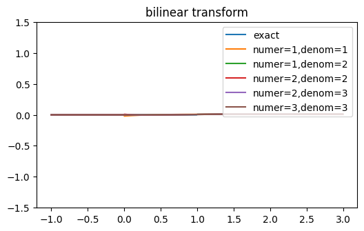
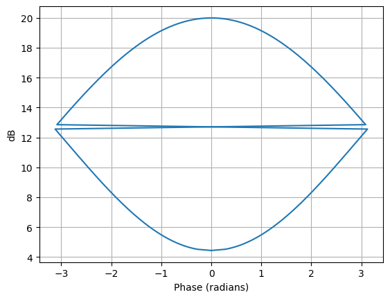
Note, some higher order approximations can be unstable. For example, the step-response of exp(-s) using a bilinear transformation is unstable for order 3 Pade approximation as in the following figure.

approximate_hyperbolic_trig(method, order, numer_order) approximates hyperbolic trig. functions with rational functions. This expands hyperbolic trig. functions using expand_hyperbolic_trig and then uses approximate_exp. For example:
```
>>> cosh(s).approximate_hyperbolic_trig(order=1)
2 - s   s + 2
───── + ─────
s + 2   2 - s
```
approximate_fractional_power(method, order) approximates s**a where a is fractional with a rational function.
approximate_numer_order(order) approximate expression by reducing order
of numerator to specified order
approximate_denom_order(order) approximate expression by reducing order
of denominator to specified order
approximate_order(order) approximate expression by reducing order to specified order
approximate(method, order, numer_order) applies many of the approximations.
prune_HOT(degree) prunes higher order terms if expression is a polynomial so that resultant approximate expression has the desired degree.

The default approximation method, and the only supported method at present, is a Pade approximant.

Parameter estimation¶

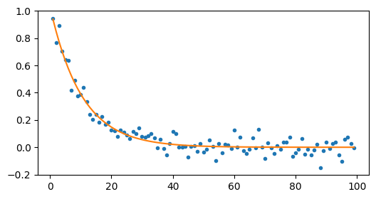
Expression parameters can be estimated using non-linear least squares optimization. This is performed by the estimate() method. For example:

>>> from numpy import arange
>>> from numpy.random import randn
>>> e = expr('a * exp(-t  / tau) * u(t)')
>>> tv = arange(1, 100)
>>> vv = e.subs({'a': 1, 'tau': 10}).evaluate(tv) + randn(len(tv)) * 0.05
>>> results = e.estimate(tv, vv, ranges={'a': (0, 10), 'tau': (1, 20)})
>>> results.params
{'a': 1.0295857498103738, 'tau': 9.617626581003838}
>>> results.rmse
0.0022484512868559342

Here’s another example using the frequency domain:

>>> e = expr('a * exp(-t  / tau) * u(t)')
>>> E = e(f)
>>> fv = arange(100)
>>> Vv = E.subs({'a': 1, 'tau': 10}).evaluate(fv)
>>> results = E.estimate(fv, Vv, ranges={'a': (0, 10), 'tau': (1, 20)})
>>> results.params
{'a': 0.999999482934574, 'tau': 10.000006318373696}
>>> results.rmse
1.3283205831942986e-14

The first argument to the estimate() method is a NumPy array of values for the dependent variable and the second argument is a NumPy array of values for the independent variable.

The ranges argument is a dictionary of search ranges (specified as a tuple) for each unknown parameter in the expression. For the curve fitting methods, the average of each search range is used as the initial guess.

estimate() has a method argument. This can be brute, lm, dogbox, Nelder-Mead, Powell, trf (default), and many others. See SciPy scipy.optimize.curve_fit, scipy.optimize.brute, and scipy.optimize.minimize for other methods and parameters. Note, the brute method is good for finding a global optimum but its execution time is exponential in the number of parameters.

A typical application is finding the model parameters given measured impedance data. For example, consider a series R, L, C network model with impedance measurements stored in an array Zv evaluated at frequencies specified by a frequency array fv. The model parameters can be estimated using:

>>> (R('R') + L('L') + C('C')).Z.estimate(fv, Zv,
... {'R': (10, 100), 'C': (1e-9, 1e-6), 'L': (1e-6, 100e-6)}).params

The dictionary argument specifies the search ranges for each parameter.

The estimate() method also has an iterations argument. If this is greater than 1, then it controls the number of iterations to perform while trying to remove outliers from the data. For example:

>>> q = expr('x * 3 + a', var='x')
>>> xv = arange(10)
>>> yv = q.subs('a', 4).evaluate(xv)
>>> y[5] = -100
>>> a = q.estimate(xv, yv)
>>> a.params
{'a': -7.899999937589999}
>>> a = q.estimate(xv, yv, iterations=5)
>>> a.params
{'a': 3.999999999999999}

Assumptions¶

SymPy relies on assumptions to help simplify expressions. In addition, Lcapy requires assumptions to help determine inverse Laplace transforms.

There are several attributes for determining assumptions:

is_dc – constant
is_ac – sinusoidal
is_causal – zero for \(t < 0\)
is_unknown – unknown for \(t < 0\)
is_real – real
is_complex – complex
is_positive – positive
is_integer – integer

For example:

>>> t.is_complex
False
>>> s.is_complex
True

The ac, dc, causal, and unknown assumptions are lazily determined. If unspecified, they are inferred prior to a Laplace transform.

Assumptions for symbols¶

The more specific the assumptions are, the easier it is for SymPy to solve an expression. For example:

>>> C_1 = symbol('C_1', positive=True)

is more appropriate for a capacitor value than:

>>> C_1 = symbol('C_1', complex=True)

Notes:

By default, the symbol and expr functions assume positive=True unless real=True or positive=False are specified.

SymPy considers variables of the same name but different assumptions to be different. This can cause much confusion since the variables look identical when printed. To avoid this problem, Lcapy creates a symbol cache for each circuit. The assumptions associated with the symbol are from when it was created.

The list of explicit assumptions for an expression can be found from the assumptions attribute. For example:

>>> a = 2 * t + 3
>>> a.assumptions
{'real': True}

The assumptions0 attribute shows all the assumptions assumed by SymPy.

Assumptions for inverse Laplace transform¶

Lcapy uses the \(\mathcal{L}_{-}\) unilateral Laplace transform (see Laplace transforms). This ignores the function for \(t <0\) and thus the unilateral inverse Laplace transform cannot determine the result for \(t <0\) unless it has additional information. This is provided using assumptions:

unknown says the signal is unknown for \(t < 0\). This is the default.
causal says the signal is zero for \(t < 0\).
damped_sin says to write response of a second-order system as a damped sinusoid.

For example:

>>> H = 1 / (s + 2)
>>> H(t)
 -2⋅t
e      for t ≥ 0

>>> H(t, causal=True)
 -2⋅t
e    ⋅Heaviside(t)

>>> h = cos(6 * pi * t)
>>> H = h(s)
>>> H
    s
──────────
 2       2
s  + 36⋅π
>>> H(t)
{cos(6⋅π⋅t)  for t ≥ 0

Discrete-time approximation¶

A continuous-time signal can be approximated by a discrete-time signal using the discretize() method. There are many methods but no universally best method since there is a trade-off between accuracy and stability.

The simplest method samples the continuous-time signal:

\[v[n] = v(n \Delta t).\]

However, this method does not work if the continuous-time signal has Dirac deltas. An example is the impulse response of a transfer function that is a pure delay or is not-strictly proper.

Other methods instead approximate the Laplace transform of the continuous-time signal in the Z-domain, and inverse Z-transform the result. These methods use different approximations for \(s = \ln(z) / \Delta t\). For example, the bilinear transform uses:

\[s = \frac{2}{\Delta t} \frac{1 - z^{-1}}{1 + z^{-1}}.\]

With an impulse response, it is common to scale the discrete-time approximation by \(\Delta t\), i.e.,

\[h[n] = \Delta t \; h(n \Delta t).\]

This corrects the scaling when approximating a continuous-time convolution integral by a discrete-time convolution sum. Lcapy makes this scaling decision on the basis of the expression quantity. If the expression is an admittance, impedance, or transfer function, the time signal is treated as an impulse response and so the \(\Delta t\) scaling is applied.

The default discretization method is ‘bilinear’. Other methods are:

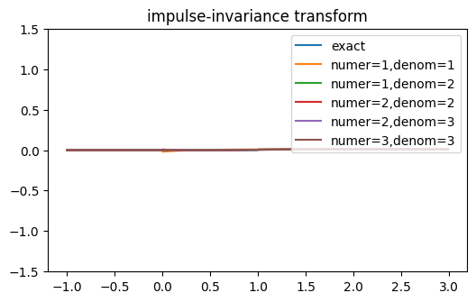
‘impulse-invariance’ samples the impulse response (using \(t = n \Delta t\)) and then converts to the Z-domain. It does not work with transfer functions that are not strictly proper (high-pass, band-pass) since these have impulse responses with Dirac deltas that cannot be be sampled. It requires the sampling frequency to be many times the system bandwidth to avoid aliasing.
‘bilinear’, ‘tustin’, ‘trapezoidal’ uses \(s = \frac{2}{\Delta t} (1 - z^{-1}) / (1 + z^{-1})\). This is equivalent to trapezoidal integration. The overall result is divided by \(\Delta t\).
‘generalized-bilinear’, ‘gbf’ uses \(s = \frac{1}{\Delta t} \frac{1 - z^{-1}}{\alpha + (1 - \alpha) z^{-1})}\) (\(\alpha = 0\) corresponds to forward Euler, \(\alpha = 0.5\) corresponds to bilinear, and \(\alpha = 1\) corresponds to backward Euler). The overall result is divided by \(\Delta t\).
‘euler’, ‘forward-diff’, ‘forward-euler’ uses \(s = \frac{1}{\Delta t} (1 - z^{-1}) / z^{-1}\). The overall result is divided by \(\Delta t\).
‘backward-diff’, ‘backward-euler’ uses \(s = \frac{1}{\Delta t} (1 - z^{-1}).\) The overall result is divided by \(\Delta t\).
‘simpson’ uses \(s = \frac{3}{\Delta t} (z^2 - 1) / (z^2 + 4 z + 1)\). This is equivalent to integration with Simpsons’s rule. The overall result is divided by \(\Delta t\). Note, this method can be more accurate but doubles the order and can lead to instability.
‘matched-Z’, ‘zero-pole-matching’ matches poles and zeros where \(s + \alpha = (1 - \exp(-\alpha \Delta t) / z)\). The overall result is divided by \(\Delta t\). When the expression has no zeros, the matched-Z and impulse invariance methods are equivalent.

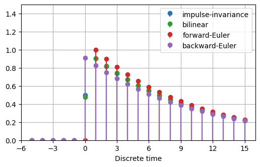
The following figure compares the impulse responses computed using some of these methods for a continuous-time impulse response \(\exp(-t) u(t)\). The matched-Z method gives the same answer as the impulse-invariance method since the Laplace transform of the impulse response has no zeros. For this example, the bilinear and impulse-invariance methods give the same response for \(n > 0\).

Plotting¶

Lcapy can generate many types of plot, including Bode plots, Nyquist plots, pole-zero plots, and lollipop (stem) plots. Labels are automatically generated but can be changed.

Expressions have a plot() method. Each domain has different behaviour. Here’s an example:

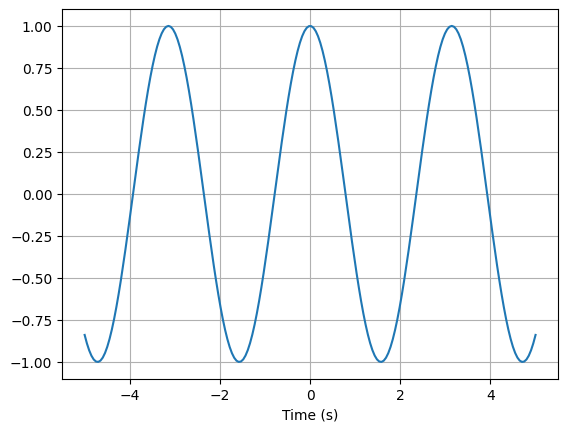
>>> cos(2 * t).plot()

You can control the range for the time values using a tuple:

>>> cos(2 * t).plot((-5, 5))

Alternatively, a NumPy array can be used:

>>> from numpy import linspace
>>> vt = linspace(-5, 5, 200)
>>> cos(2 * t).plot(vt)

The returned value from the plot() method is a Matplotlib axes object (or a tuple if more than one set of axes are used, say for a magnitude/phase plot). This is useful to overlay plots, for example:

>>> from numpy import linspace
>>> vt = linspace(-5, 5, 200)
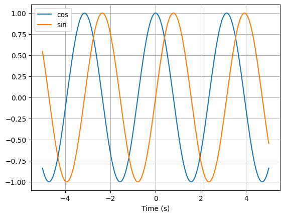
>>> axes = cos(2 * t).plot(vt, label='cos')
>>> sin(2 * t).plot(vt, label='sin', axes=axes)
>>> axes.legend()

You can create your own Matplotlib axes and use this for plotting:

>>> from matplotlib.pyplot import subplots
>>> from numpy import linspace
>>> vt = linspace(-5, 5, 200)
>>> figs, axes = subplots(1)
>>> cos(2 * t).plot(vt, axes=axes, label='cos')
>>> sin(2 * t).plot(vt, axes=axes, label='sin')
>>> axes.legend()

Finally, you can manage all the plotting yourself, for example:

>>> from matplotlib.pyplot import subplots
>>> from numpy import linspace
>>> vt = linspace(-5, 5, 200)
>>> figs, axes = subplots(1)
>>> axes.plot(vt, cos(2 * t).evaluate(vt), label='cos')
>>> axes.plot(vt, sin(2 * t).evaluate(vt), label='sin')
>>> axes.legend()

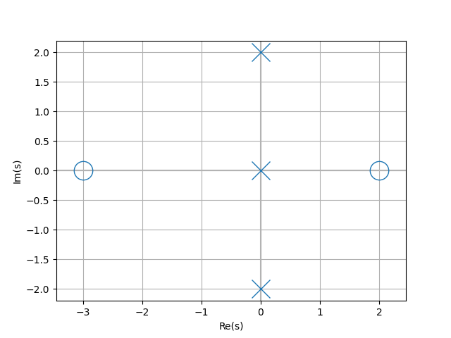
Pole-zero plots¶

The plot() method for Laplace-domain expressions generates a pole-zero plot, for example:

from lcapy import s, j, transfer
from matplotlib.pyplot import savefig

H = transfer((s - 2) * (s + 3) / (s * (s - 2 * j) * (s + 2 * j)))
H.plot()

savefig('tf1-pole-zero-plot.png')

Frequency-domain plots¶

Here’s an example of the plot() method for Fourier-domain expressions:

from lcapy import s, j, pi, f, transfer, j2pif
from matplotlib.pyplot import savefig
from numpy import logspace

# Note, this has a marginally stable impulse response since it has a
# pole at s = 0.
H = transfer((s - 2) * (s + 3) / (s * (s - 2 * j) * (s + 2 * j)))

fv = logspace(-1, 3, 400)
H(j2pif).dB.plot(fv, log_scale=True)

savefig('tf1-bode-plot.png')

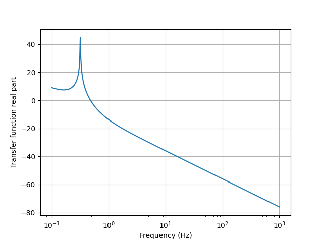
The type of plot for complex frequency-domain expressions is controlled by the plot_type argument. By default this is dB-phase for complex expressions which plots both the magnitude as dB and the phase. Other choices are real, imag, magnitude, phase, real-imag, magnitude-phase, dB, degrees, and radians.

Frequencies are shown on a linear scale by default. A logarithmic scale is used if log_frequency=True is specified.

Magnitudes are shown on a linear scale by default. A logarithmic scale is used if log_magnitude=True is specified.

Phases are wrapped unless unwrap=True is specified to avoid discontinuities of math:pi.

The frequency domain plot() method returns the axes used in the plot. If there are two sets of axes, such as for a magnitude/phase or real/imaginary plot, these are returned as a tuple. For example:

>>> A = 1 / (j * 2 * pi * f)
>>> axm, axp = A.plot()

>>> A = 1 / (j * 2 * pi * f)
>>> ax = abs(A).plot()

Bode plots¶

Bode plots are similar to frequency domain plots but plot both the magnitude (in dB) and the phase (in radians) as a function of logarithmic frequency. The phase is unwrapped by default to avoid discontinuities of \(\pi\).

from matplotlib.pyplot import savefig
from lcapy import *

H = 1 / (s**2 + 20*s + 10000)

H.bode_plot((1, 1000))

savefig(__file__.replace('.py', '.png'), bbox_inches='tight')

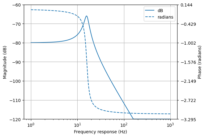
By default, a Bode plot of a Laplace domain expression is shown with linear frequencies (in hertz). This can be changed to angular frequencies (in radians) using the var=omega argument to the bode_plot() method.

The frequency response of Laplace domain expressions is calculated using the substitution \(s = j \omega\). Note, this does not correctly calculate the DC component for expressions that have an unstable impulse response.

Nyquist plots¶

Nyquist plots plot the imaginary part of a frequency response expression against the real part.

from matplotlib.pyplot import savefig
from lcapy import *

H = 10 * (s + 1) * (s + 2) / ((s - 3) * (s - 4))

H.nyquist_plot((-100, 100))

savefig(__file__.replace('.py', '.png'), bbox_inches='tight')

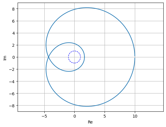
By default, the points on the plot are geometrically spaced; this can be disabled with log_frequency=False.

The unit circle is shown by default. This can be disabled with unitcircle=False.

Nichols plots¶

Nichols plots plot the magnitude of the frequency response in dB versus the phase of the frequency response in radians.

from matplotlib.pyplot import savefig
from lcapy import *

H = 10 * (s + 1) * (s + 2) / ((s - 3) * (s - 4))

H.nichols_plot((-100, 100))

savefig(__file__.replace('.py', '.png'), bbox_inches='tight')

By default, the points on the plot are geometrically spaced; this can be disabled with log_frequency=False.

Phasor plots¶

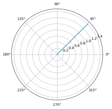
Phasors are plotted on a polar graph, for example:

>>> phasor(1 + j).plot()

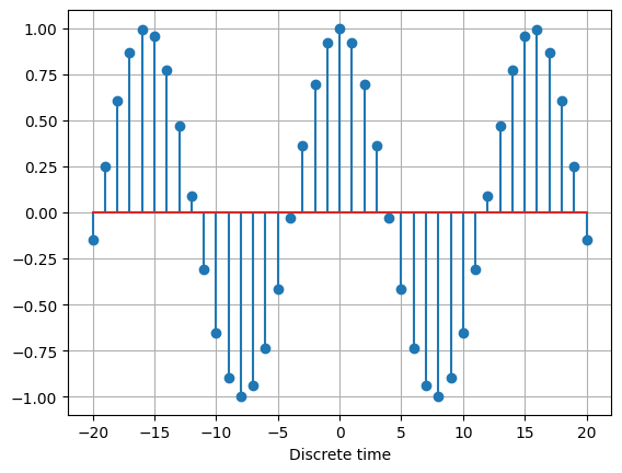
Discrete-time plots¶

Discrete-time signals are plotted as stem (lollipop) plots, for example:

>>> cos(2 * n * 0.2).plot()

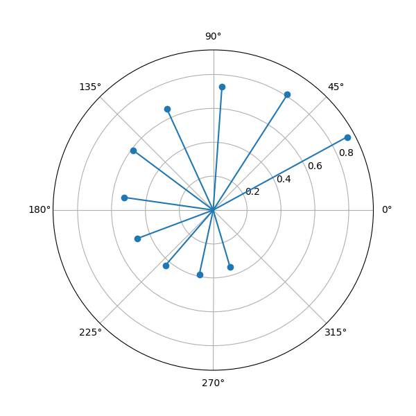
Complex discrete-time signals can also be plotted in polar format, for example:

>>> x = 0.9**n * exp(j * n * 0.5)
>>> x.plot((1, 10), polar=True)

Dirac deltas¶

Dirac deltas in a time domain or discrete-time domain expression are plotted as arrows. For example:

from matplotlib.pyplot import savefig
from lcapy import *

nexpr(1).DTFT().remove_images((-5, 5)).subs(dt, 1).plot((-5, 5))

savefig(__file__.replace('.py', '.png'), bbox_inches='tight')

Plot customisation¶

The plot() method has a number of generic keyword arguments to customise the plots. These include:

xlabel sets the xlabel string
ylabel sets the ylabel string
title sets the title string

For example:

>>> H = s / (s + 2)
>>> H.plot(xlabel=r'$\sigma$', ylabel=r'$\omega$', title='Pole zero plot')

Alternatively, this can be achieved using:

>>> H = s / (s + 2)
>>> ax = H.plot()
>>> ax.set_xlabel(r'$\sigma`)
>>> ax.set_ylabel(r'$\omega`)
>>> ax.set_title('Pole zero plot')

Other keyword arguments are passed to the matplotlib plot routines. For example:

>>> H = s / (s + 2)
>>> H.plot(markersize=20)

The best way to customise plots is to create a matplotlib style file. For example,

>>> from matplotlib.pyplot import style
>>> style.use('polezero.mplstyle')
>>> H = s / (s + 2)
>>> H.plot()

where polezero.mplstyle might contain

lines.markersize = 20

font.size = 14

Matplotlib has many pre-defined styles, see https://matplotlib.org/stable/gallery/style_sheets/style_sheets_reference.html .

Parameterization¶

Lcapy can parameterize an expression into zero-pole-gain (ZPK) form with the parameterize_ZPK() method. For example:

>>> H = (5*s**2 + 5) / (s**2 + 5*s + 4)
>>> H1, defs = H.parameterize_ZPK()
>>> H1
   (s - z₁)⋅(s - z₂)
K⋅───────────────────
  (-p₁ + s)⋅(-p₂ + s)
>>> defs
{K: 5, p1: -1, p2: -4, z1: -ⅉ, z2: ⅉ}

Note, SymPy likes to print p before s and hence -p1 + s rather than s - p1.

defs is a dictionary of definitions; it can be substituted into the parameterized expression to obtain the original expression:

>>> H1.subs(defs)
     3
────────────
 2
z  + 5⋅z + 4

Lcapy can parameterize a number of first order, second order, and third order s-domain expressions into common forms. For example:

>>> H1 = 3 / (s + 2)
>>> H1p, defs = H1.parameterize()
>>> H1p
  K
─────
α + s
>>> defs
{K: 3, alpha: 2}

Here defs is a dictionary of the parameter definitions.

The original expression can be obtained by substituting the parameter definitions into the parameterized expression:

>>> H1p.subs(defs)
  3
─────
s + 2

Here’s a second order example:

>>> H2 = 3 / (s**2 + 2*s + 4)
>>> H2p, defs = H2.parameterize()
>>> H2p
           K
───────────────────
  2               2
ω₀  + 2⋅ω₀⋅s⋅ζ + s

>>> defs
{K: 3, omega_0: 2, zeta: 1/2}

Second order systems can be parameterized in many ways. Here’s another example:

>>> H2p, defs = H2.parameterize(zeta=False)
>>> H2p
            K
───────────────────────
  2    2              2
ω₁  + s  + 2⋅s⋅σ₁ + σ₁

>>> defs
{K: 3, omega_1: √3, sigma_1: 1}

Network synthesis¶

Lcapy has experimental support for a number of network synthesis. This produces a network model from an s-domain impedance or admittance expression. There are many methods, some specifically for simple networks such as R-L networks, and more general methods including Foster and Cauer synthesis.

>>> Z = impedance((4*s**2 + 3 * s + one / 6) / (s**2 + 2 * s / 3))
>>> n = Z.network('cauerI')
>>> n
((C(1) + R(2)) | C(3)) + R(4)
>>> n.Z(s).canonical()

\(\frac{4 s^{2} + 3 s + \frac{1}{6}}{s^{2} + \frac{2 s}{3}}\)

>>> n.draw()

Note, in this example, one is used to avoid generating a floating-point number 1 / 6. An alternative approach to use quotes around the expression (see Floating point values):

>>> Z = impedance('(4*s**2 + 3 * s + 1 / 6) / (s**2 + 2 * s / 3)')

Here’s another example::

>>> n2 = Z.network('fosterI')
>>> n2
R(4) + (R(1/8) | C(12)) + C(4)
>>> n2.draw()

Special functions¶

Heaviside unit step H(t)¶

The Heaviside unit step is defined as

\[\begin{split}\mathop{\mathrm{sign}}(t) = \begin{cases} 0 & t < 0 \\ 0.5 & t = 0 \\ 1 & t > 0 \end{cases}\end{split}\]

Note, the definition H(0) = 0.5 is consistent with sign(0) = 0 (as used with SymPy and NumPy) using the relation:

\[H(t) = \frac{1}{2}(1 + \mathop{\mathrm{sign}}(t))\]

Note, there is also a related discrete-time function called unitstep.

Signum function sign(t)¶

The signum function sign(t) is defined in terms of the Heaviside function as:

\[\mathop{\mathrm{sign}}(t) = 2 \mathop{\mathrm{H}}(t) - 1\]

and thus:

\[\begin{split}\mathop{\mathrm{sign}}(t) = \begin{cases} -1 & t < 0 \\ 0 & t = 0 \\ 1 & t > 0 \end{cases}\end{split}\]

Note, there is also a related discrete-time signum function.

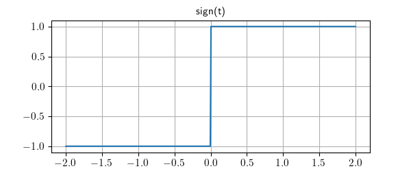
Ramp function ramp(t)¶

The rectangle function ramp(t) is defined in terms of the Heaviside step as

\[\mathop{\mathrm{ramp}}(t) = t H(t)\]

In other words

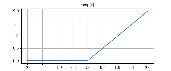
\[\begin{split}\mathop{\mathrm{ramp}}(t) = \begin{cases} 0 & t < 0 \\ t & t > 0 \end{cases}\end{split}\]

Rampstep function rampstep(t)¶

The rectangle function rampstep(t) is defined in terms of the ramp function as

\[\mathop{\mathrm{rampstep}}(t) = \mathop{\mathrm{ramp}}(t) - \mathop{\mathrm{ramp}}(t - 1)\]

or in terms of the Heaviside’s step as

\[\mathop{\mathrm{rampstep}}(t) = t H(t) - (t - 1) H(t - 1)\]

In other words

\[\begin{split}\mathop{\mathrm{rampstep}}(t) = \begin{cases} 0 & t < 0 \\ t & 0 \le t \le 1 \\ 1 & t > 1 \end{cases}\end{split}\]

Rectangle function rect(t)¶

The rectangle function rect(t) is defined in terms of the Heaviside step as

\[\mathop{\mathrm{rect}}(t) = H(t + 1 / 2) - H(t - 1 / 2)\]

With the assumption H(0) = 0 then rect(0.5) = 0.5. In other words

\[\begin{split}\mathop{\mathrm{rect}}(t) = \begin{cases} 0 & t < -0.5 \\ -0.5 & t = 0.5 \\ 1 & -0.5 \lt t \lt 0.5 \\ 0.5 & t = 0.5 \\ 0 & t > 0.5 \end{cases}\end{split}\]

Note, there is also a related discrete-time rectangle dtrect defined in terms of the discrete-time unit step function.

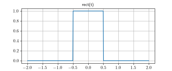
A casual rect function can be created by a shift of 0.5.

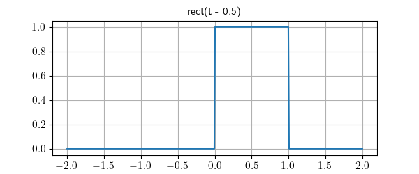
Triangle function tri(t)¶

The triangle function tri(t) is the convolution of rect(t) and rect(t).

It can be described in terms of the ramp function as

\[\mathop{\mathrm{tri}}(t) = \mathop{\mathrm{ramp}}(t + 1) - 2 \mathop{\mathrm{ramp}}(t) + \mathop{\mathrm{ramp}}(t - 1)\]

or in terms of Heaviside’s step as

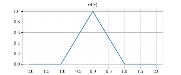
\[\mathop{\mathrm{tri}}(t) = (t + 1) H(t + 1) - 2 t H(t) + (t - 1) H(t - 1)\]

A casual triangle function can be created by a shift of 1.

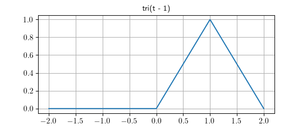
Trapezoid function trap(t, alpha)¶

The trapezoid function trap(t, alpha) is the convolution of rect(t / alpha) and rect(t). The parameter alpha is the normalized rise/fall time. When alpha = 0 it is equivalent to rect(t) and when alpha = 1 it is equivalent to tri(t).

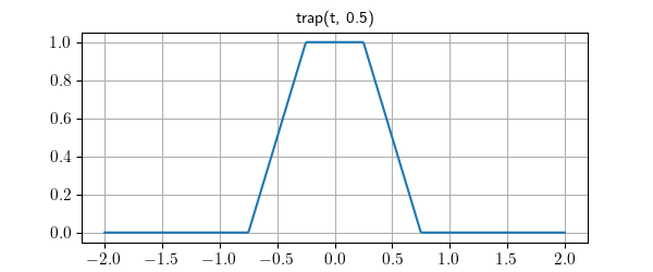
A casual trap function can be created by a shift of (1 + alpha) / 2.

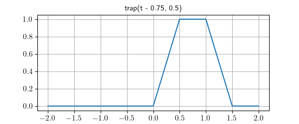
Cardinal sine function sinc(t)¶

Lcapy uses the normalized form of the sinc function (cardinal sine),

\[\mathop{\mathrm{sinc}}(t) = \mathop{\mathrm{sincn}}(t) = \frac{\sin(\pi t)}{\pi t}.\]

This definition is the same as NumPy but SymPy uses the unnormalized form

\[\mathop{\mathrm{sinc}}(t) = \mathop{\mathrm{sincu}}(t) = \frac{\sin(t)}{t}.\]

Note, Lcapy prints sinc as sincn due to a bug in SymPy. This is likely to change in the future.

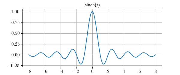
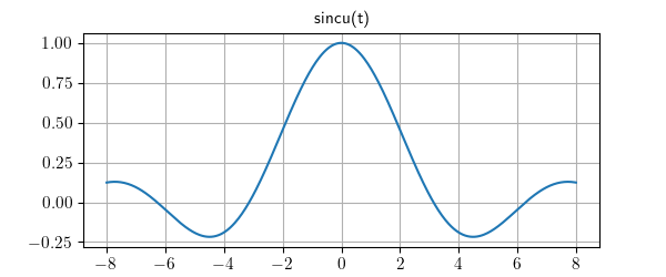
Periodic sinc function psinc(M, t)¶

The periodic sinc psinc function is defined as

\[\mathop{\mathrm{psinc}}(M, t) = \frac{\sin(M \pi t)}{M \sin(\pi t)}\]

It is sometimes called the aliased sinc function and is similar to the Dirichlet function, usually defined as

\[D_M(t) = \frac{\sin(M t / 2)}{M \sin(t / 2)}\]

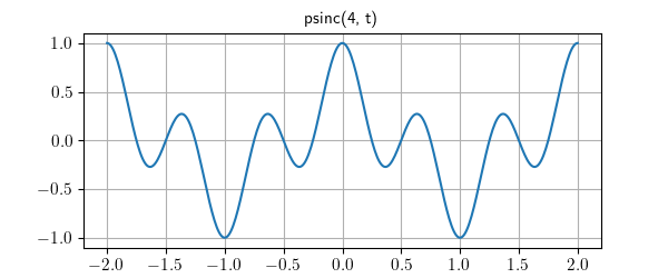
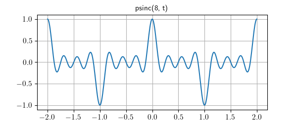
Note, psinc(2, t) is equivalent to cos(pi * t).

Discrete-time unit step u[n]¶

The discrete-time unit step is defined as

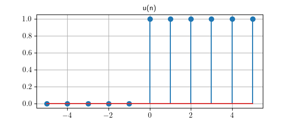
\[\begin{split}\mathop{\mathrm{u}}[n] = \begin{cases} 0 & n < 0 \\ 1 & n \gt 0 \end{cases}\end{split}\]

Discrete-time unit impulse delta[n]¶

The discrete-time unit impulse is defined as

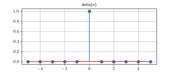
\[\begin{split}\mathop{\delta}[n] = \begin{cases} 0 & n < 0 \\ 1 & n = 0 \\ 0 & n > 0 \end{cases}\end{split}\]

Discrete-time rectangle function rect[n]¶

The discrete-time rectangle function rect[n] is defined in terms of the discrete-time unit step function as:

\[\mathop{\mathrm{rect}}[n] = \mathop{\mathrm{u}}[n + 1 / 2] - \mathop{\mathrm{u}}[n - 1 / 2]\]

With this definition:

\[\begin{split}\mathop{\mathrm{rect}}[n] = \begin{cases} 0 & n < -0.5 \\ 1 & -0.5 \le n \lt 0.5 \\ 0 & n > 0.5 \end{cases}\end{split}\]

Notes:

Lcapy converts rect(n) to dtrect(n) for discrete-time signals and prints it as rect[n].
dtrect(n/N) produces a symmetrical result when N is odd. When N is even, there is one more non-zero value for negative n compared to positive n.
The internal name dtrect may change when I can think of something better.

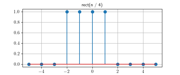
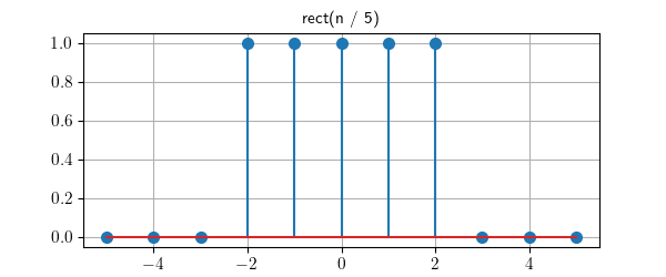
Discrete-time signum function sign[n]¶

The discrete-time signum function sign[n] is defined in terms of the discrete-time unit step function as:

\[\mathop{\mathrm{sign}}[n] = 2 \mathop{\mathrm{u}}[n] - 1\]

and thus:

\[\begin{split}\mathop{\mathrm{sign}}[n] = \begin{cases} -1 & n < 0 \\ 1 & n \ge 0 \end{cases}\end{split}\]

Notes:

Lcapy converts sign(n) to dtsign(n) for discrete-time signals and prints it as sign[n].
The internal name dtsign may change when I can think of something better.

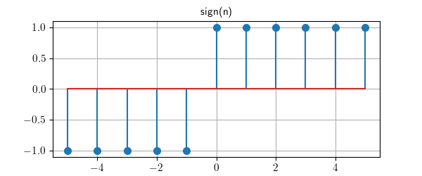
Expression manipulation tips¶

SymPy expressions¶

Lcapy does not support all the SymPy functions. However, the underlying SymPy expression can be obtained using the sympy attribute of an Lcapy expression. For example:

>>> a = 2 * t + 3
>>> a.sympy
2⋅t + 3

The result can then be converted back to an Lcapy expression using the expr() function.

Functions¶

Lcapy functions are a wrapper around a SymPy function that converts Lcapy expression arguments into SymPy expressions and converts the result into an Lcapy expression.

Lcapy does not explicitly support all the SymPy functions. However, a SymPy function can be made into an Lcapy function using the Function class, for example:

>>> import sympy
>>> from lcapy import Function
>>> gamma = Function(sympy.Gamma)

The Integral and Derivative functions are not evaluated unlike the corresponding integrate and diff functions. The evaluation can be performed using the doit() method.

Undefined functions can be created by passing a string name to Function:

>>> from lcapy import Function
>>> g = Function('g')
>>> g
g
>>> g(t)
g(t)
>>> g(t)(s)
G(s)

Assumptions¶

Correct assumptions are required for Lcapy (and SymPy) to simplify expressions. Note, there are two sets of assumptions. Firstly there are assumptions that Lcapy maintains for an Lcapy expression. These can be found with the assumptions attribute. Secondly, there are assumptions that SymPy uses for a symbol. These can be found with the assumptions0 attribute. For example:

>>> t.assumptions
{'real': True}

>>> t.assumptions0
{'real': True,
'complex': True,
'infinite': False,
'hermitian': True,
'commutative': True,
'finite': True,
'imaginary': False,
'extended_real': True}

>>> x = symbol('x', positive=True, integer=True)
>>> x.assumptions0
{'positive': True,
'complex': True,
'nonpositive': False,
'infinite': False,
'nonzero': True,
'hermitian': True,
'extended_nonzero': True,
'zero': False,
'real': True,
'commutative': True,
'extended_negative': False,
'negative': False,
'extended_nonnegative': True,
'extended_nonpositive': False,
'finite': True,
'imaginary': False,
'nonnegative': True,
'extended_real': True,
'extended_positive': True,
'integer': True,
'algebraic': True,
'rational': True,
'irrational': False,
'noninteger': False,
'transcendental': False}

Note, the symbol x has positive, integer, real, and complex attributes since it is represents a positive integer value, integers are in the set of reals, and the reals are within the set of complex numbers. However, it is not a complex value:

>>>  x.is_complex
False

Parameterization¶

Symbolic expressions can get unwieldy. One approach is to parameterize an expression using the parameterize() method, perform manipulations, and then substitute for the parameter definitions.