Networks
Lcapy supports one-port and two-port networks.
One-port networks
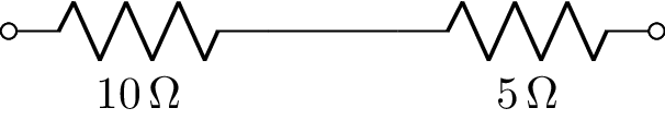
One-port networks are creating by combining one-port components in series or parallel, for example, here’s an example of resistors in series
>>> from lcapy import R
>>> R1 = R(10)
>>> R2 = R(5)
>>> Rtot = R1 + R2
>>> Rtot
R(10) + R(5)
Here R(10) creates a 10 ohm resistor and this is assigned to the variable R1. Similarly, R(5) creates a 5 ohm resistor and this is assigned to the variable R2. Rtot is the name of the network formed by connecting R1 and R2 in series.
>>> Rtot.draw()
Network components
C capacitor
CPE constant phase element
Damper mechanical damper
FeriteBead ferrite bead (lossy inductor)
G conductance
I arbitrary current source
i arbitrary time-domain current source
Iac ac current source (default angular frequency \(\omega_0\))
Idc dc current source
Inoise noise current source
Istep step current source
L inductor
Mass mass
O open-circuit
R resistor
NR noiseless resistor (this is generated by the noisy() method)
Spring spring
sV s-domain voltage source
sI s-domain current source
V arbitrary voltage source
v arbitrary time-domain voltage source
Vac ac voltage source (default angular frequency \(\omega_0\))
Vdc dc voltage source
Vnoise noise voltage source
Vstep step voltage source
Xtal crystal
W wire
Y generalized admittance
Z generalized impedance
Network attributes
Each network oneport has a number of attributes, including:
Voc transform-domain open-circuit voltage
Isc transform-domain short-circuit current
I transform-domain current through network terminals (zero by definition)
voc t-domain open-circuit voltage
isc t-domain short-circuit current
isc t-domain current through network terminals (zero by definition)
B susceptance
G conductance
R resistance
X reactance
Y admittance
Z impedance
Ys s-domain generalized admittance
Zs s-domain generalized impedance
y t-domain impulse response of admittance
z t-domain impulse response of impedance
is_dc DC network
is_ac AC network
is_IVP initial value problem
is_causal causal response
is_series series network
is_parallel parallel network
Here’s an example:
>>> from lcapy import R, V
>>> n = V(20) + R(10)
>>> n.Voc
20
──
 s
>>> n.voc
20
>>> n.Isc
2
─
s
>>> n.isc
2
>>> n.Z
10
>>> n.Y
1/10

Network methods
circuit() create a Circuit object from the network.
describe() print a message describing how network is solved.
draw() draw the schematic.
netlist() create an equivalent netlist.
subs(subs_dict) substitutes symbolic values in the network using a dictionary of symbols subs_dict.
noisy(T=’T’) create noisy model where resistors are replaced with a noiseless resistor and a noise voltage source.
Network functions
series() connect one-port components in series. This is similar to Ser() but is robust to None components and single components in series.
parallel() connect one-port components in parallel. This is similar to Par() but is robust to None components and single components in parallel.
ladder() connect one-port components as a one-port ladder network. This is an alternating sequence of series and parallel connections. For example:
>>> ladder(R(1), C(2), R(3))
R(1) + (C(1) | R(3))
>>> ladder(None, C(2), R(3), C(3))
C(2) | (R(3) + C(3))
Network simplification
A network can be simplified (if possible) using the simplify method. For example, here’s an example of a parallel combination of resistors. Note that the parallel operator is | instead of the usual ||.
>>> from lcapy import *
>>> Rtot = R(10) | R(5)
>>> Rtot
R(10) | R(5)
>>> Rtot.simplify()
R(10/3)
The result can be performed symbolically, for example:
>>> from lcapy import *
>>> Rtot = R('R_1') | R('R_2')
>>> Rtot
R(R_1) | R(R_2)
>>> Rtot.simplify()
R(R_1*R_2/(R_1 + R_2))
>>> Rtot.simplify()
R(R₁) | R(R₂)
Here’s another example using inductors in series
>>> from lcapy import *
>>> L1 = L(10)
>>> L2 = L(5)
>>> Ltot = L1 + L2
>>> Ltot
L(10) + L(5)
>>> Ltot.simplify()
L(15)
Finally, here’s an example of a parallel combination of capacitors
>>> from lcapy import *
>>> Ctot = C(10) | C(5)
>>> Ctot
C(10) | C(5)
>>> Ctot.simplify()
C(15)
Norton and Thevenin transformations
A Norton or Thevenin equivalent network can be created using the norton or thevenin methods. For example:
>>> from lcapy import Vdc, R
>>> a = Vdc(1) + R(2)
>>> a.norton()
G(1/2) | Idc(1/2)
Network schematics
Networks are drawn with the draw() method. Here’s an example:
>>> from lcapy import R, C, L
>>> ((R(1) + L(2)) | C(3)).draw()
Here’s the result:
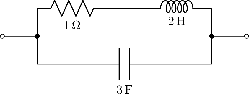
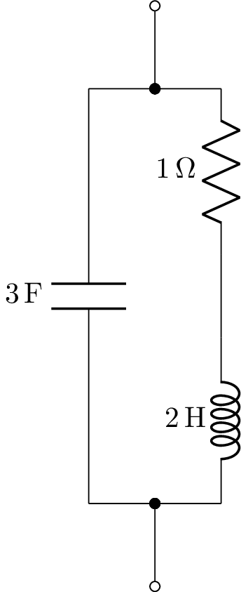
By default, one port networks are drawn with a horizontal layout. This can be changed to a vertical layout or as a ladder layout using the form argument to the draw() method.
Here’s an example of a vertical layout,
>>> from lcapy import R, C, L
>>> ((R(1) + L(2)) | C(3)).draw(form='vertical')
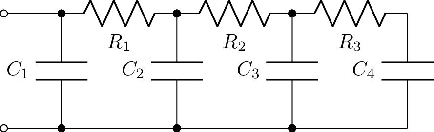
Here’s an example of a network drawn with ladder layout,
>>> from lcapy import R, C
>>> n = C('C1') | (R('R1') + (C('C2') | (R('R2') + (C('C3') | (R('R3') + C('C4'))))))
>>> n.draw(form='ladder')
The s-domain model can be drawn using:
>>> from lcapy import R, C, L
>>> ((R(1) + L(2)) | C(3)).s_model().draw()
This produces:
Internally, Lcapy converts the network to a netlist and then draws the netlist. The netlist can be found using the netlist method, for example,
>>> from lcapy import R, C, L
>>> print(((R(1) + L(2)) | C(3)).netlist())
yields:
W 1 2; right=0.5
W 2 4; up=0.4
W 3 5; up=0.4
R1 4 6 1; right
W 6 7; right=0.5
L1 7 5 2; right
W 2 8; down=0.4
W 3 9; down=0.4
C1 8 9 3; right
W 3 0; right=0.5
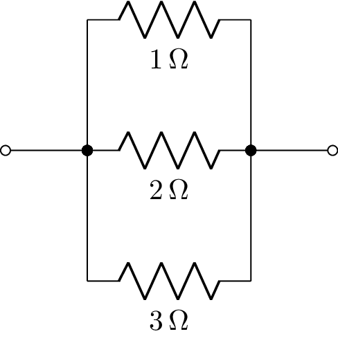
To create a schematic with multiple components in parallel, use Par. For example,
from lcapy import R, C, L, Par
N = Par(R(1), R(2), R(3))
N.draw('par3.png')
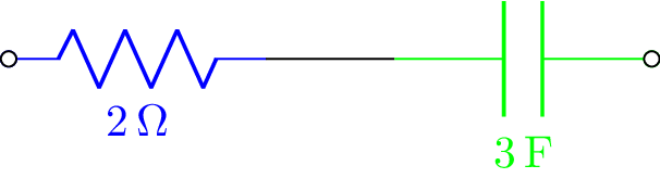
The network components have optional keyword arguments (kwargs) that specify schematic attributes, for example:
>>> (R(2, color='blue') + C(3, color='green')).draw()
Network synthesis
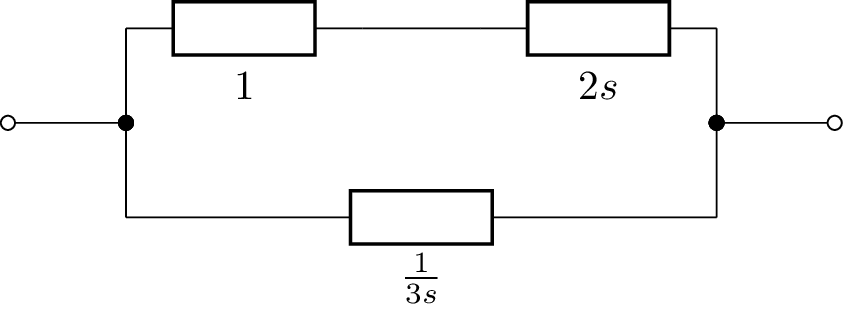
Networks can be created using network synthesis techniques given an impedance or admittance expression, for example:
>>> Z = impedance(4*s**2 + 3 * s + 1 / 6) / (s**2 + 2 * s / 3)
>>> Z.network()
((C(1) + R(2)) | C(3)) + R(4)
>>> Z.network().Z(s).canonical()
\(\frac{4 s^{2} + 3 s + \frac{1}{6}}{s^{2} + \frac{2 s}{3}}\)
For more details, see Network synthesis.
Random networks
Networks can be randomly generated with the random_network function. This is useful for automated exam question generation. Here’s an example:
>>> from lcapy import random_network
>>> net = random_network(num_resistors=4, num_capacitors=0, num_inductors=0, num_voltage_sources=2, kind='dc')
This example generates a DC network with four resistors, two-voltage sources, and no capacitors or inductors. The kind argument can be ac, dc, or transient. The number of parallel connections can be specified with the num_parallel argument.
If you want to assign integer random values for the component values, use something like:
>>> defs = {}
... for p in net.params:
...    defs[p] = int((rand(1) + 1) * 10)
... net2 = net.subs(defs)
Network analysis examples
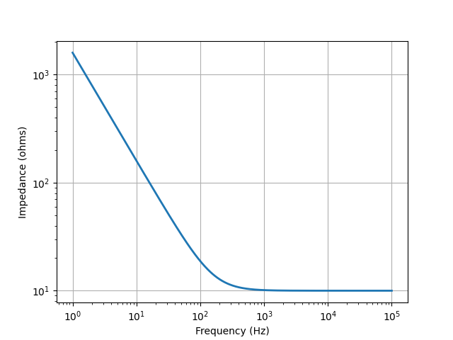
Series R-C network
from lcapy import *
from numpy import logspace
from matplotlib.pyplot import figure, savefig

N = R(10) + C(1e-4)

vf = logspace(0, 5, 400)
Z = N.Z(j2pif).evaluate(vf)

fig = figure()
ax = fig.add_subplot(111)
ax.loglog(vf, abs(Z), linewidth=2)
ax.set_xlabel('Frequency (Hz)')
ax.set_ylabel('Impedance (ohms)')
ax.grid(True)

savefig('series-RC1-Z.png')
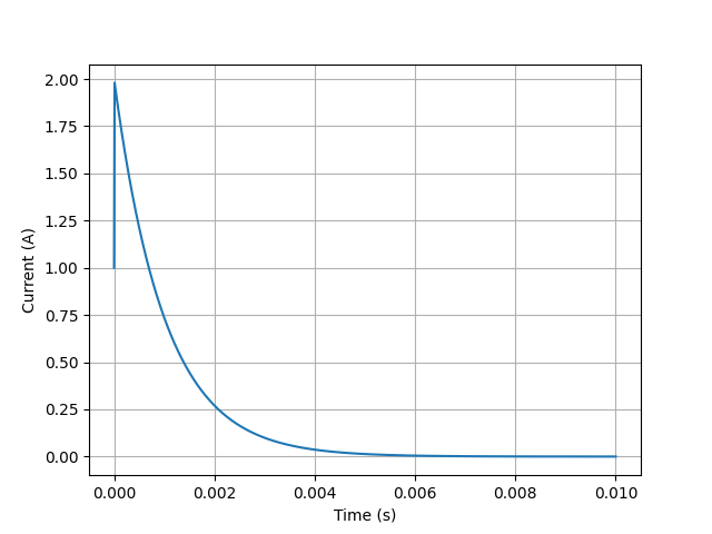
from lcapy import *
from numpy import linspace
from matplotlib.pyplot import savefig

N = Vstep(20) + R(10) + C(1e-4, 0)

vt = linspace(0, 0.01, 1000)
N.Isc(t).plot(vt)

savefig('series-VRC1-isc.png')
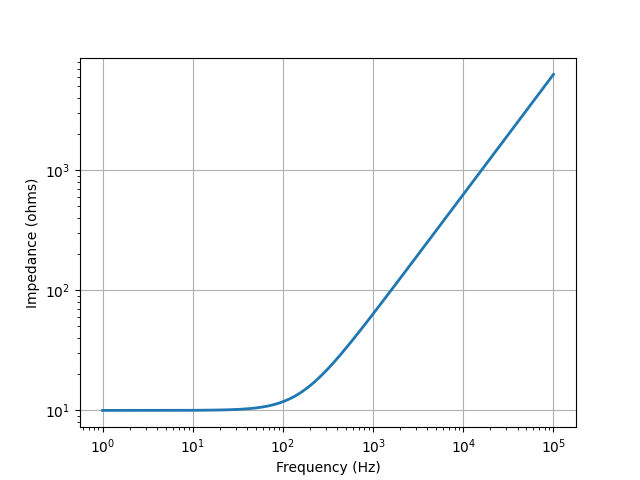
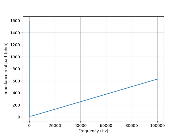
Series R-L network
from lcapy import *
from numpy import logspace
from matplotlib.pyplot import figure, savefig

N = R(10) + L(1e-2)

vf = logspace(0, 5, 400)
Z = N.Z(j2pif).evaluate(vf)

fig = figure()
ax = fig.add_subplot(111)
ax.loglog(vf, abs(Z), linewidth=2)
ax.set_xlabel('Frequency (Hz)')
ax.set_ylabel('Impedance (ohms)')
ax.grid(True)

savefig('series-RL1-Z.png')
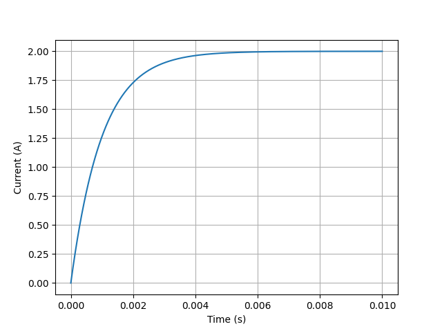
from lcapy import *
from numpy import linspace
from matplotlib.pyplot import savefig

N = Vstep(20) + R(10) + L(1e-2, 0)

vt = linspace(0, 0.01, 1000)
N.Isc(t).plot(vt)

savefig('series-VRL1-isc.png')
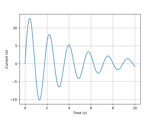
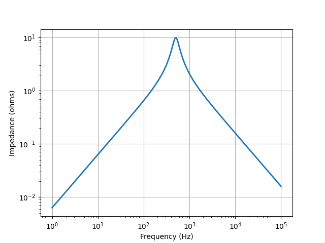
Series R-L-C network
from lcapy import *
from numpy import logspace
from matplotlib.pyplot import savefig

N = R(10) + C(1e-4) + L(1e-3)

vf = logspace(0, 5, 400)
N.Z(j2pif).magnitude.plot(vf)

savefig('series-RLC3-Z.png')
from lcapy import Vstep, R, L, C, t
from matplotlib.pyplot import savefig
from numpy import linspace

a = Vstep(10) + R(0.1) + C(0.4) + L(0.2, 0)

vt = linspace(0, 10, 1000)
a.Isc(t).plot(vt)

savefig('series-VRLC1-isc.png')
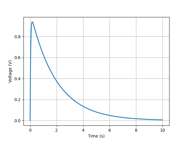
Parallel R-L-C network
from lcapy import *
from numpy import logspace
from matplotlib.pyplot import figure, savefig

N = R(10) | C(1e-4) | L(1e-3)

vf = logspace(0, 5, 400)
Z = N.Z(j2pif).evaluate(vf)

fig = figure()
ax = fig.add_subplot(111)
ax.loglog(vf, abs(Z), linewidth=2)
ax.set_xlabel('Frequency (Hz)')
ax.set_ylabel('Impedance (ohms)')
ax.grid(True)


savefig('parallel-RLC3-Z.png')
from lcapy import Istep, R, L, C, t
from matplotlib.pyplot import figure, savefig
import numpy as np

a = Istep(10) | R(0.1) | C(0.4) | L(0.2)

vt = np.linspace(0, 10, 1000)

fig = figure()
ax = fig.add_subplot(111)
ax.plot(vt, a.Voc(t).evaluate(vt), linewidth=2)
ax.set_xlabel('Time (s)')
ax.set_ylabel('Voltage (V)')
ax.grid(True)

savefig('parallel-IRLC1-voc.png')
Two-port networks
Two-port networks are represented in the Laplace domain. Basic two-ports networks can be combined to produce more complicated two-port networks.
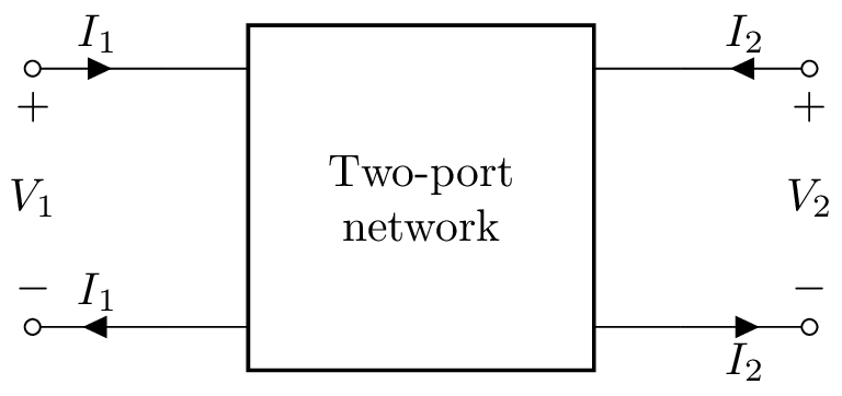
A two-port is an electrical black-box with two pairs of terminals. A pair of terminals is considered a port if the port condition is satisfied, i.e., the flow of current into one terminal is the same as the current flowing out of the other terminal.
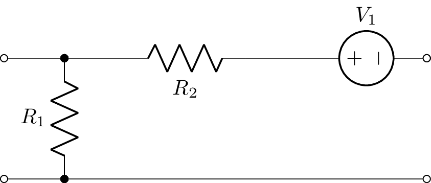
Two-port networks are usually considered to be free of independent sources, however, Lcapy uses a generalized form that has two optional independent sources. For lack of a better term, these are currently called two-port models. They consist of a 2x2 matrix describing the network parameters and a 2x1 vector describing the independent sources (see Two-port network models). For example, consider the network:
>>> tp = Shunt(R('R1')).chain(Series(R('R2') + V('V1')))
This can be drawn using:
>>> tp.draw()
This network is represented by B-parameters but can be converted to a Z-parameter model using the Zmodel attribute:
>>> ztp = tp.Zmodel
The Z-parameters are obtained with the params attribute:
>>> ztp.params

⎡R₁       R₁      ⎤
⎢                 ⎥
⎢        ⎛     R₂⎞⎥
⎢R₁  -R₁⋅⎜-1 - ──⎟⎥
⎣        ⎝     R₁⎠⎦
The sources are obtained with the sources attribute:
>>> ztp.sources

⎡0 ⎤
⎢  ⎥
⎢V₁⎥
⎢──⎥
⎣s ⎦
The system of equations can be obtained using the equation() method, for example:
>>> ztp.equation()

       ⎡R₁       R₁      ⎤        ⎡0 ⎤
⎡V₁⎤   ⎢                 ⎥ ⎡I₁⎤   ⎢  ⎥
⎢  ⎥ = ⎢        ⎛     R₂⎞⎥⋅⎢  ⎥ + ⎢V₁⎥
⎣V₂⎦   ⎢R₁  -R₁⋅⎜-1 - ──⎟⎥ ⎣I₂⎦   ⎢──⎥
       ⎣        ⎝     R₁⎠⎦        ⎣s ⎦
Basic two-port networks
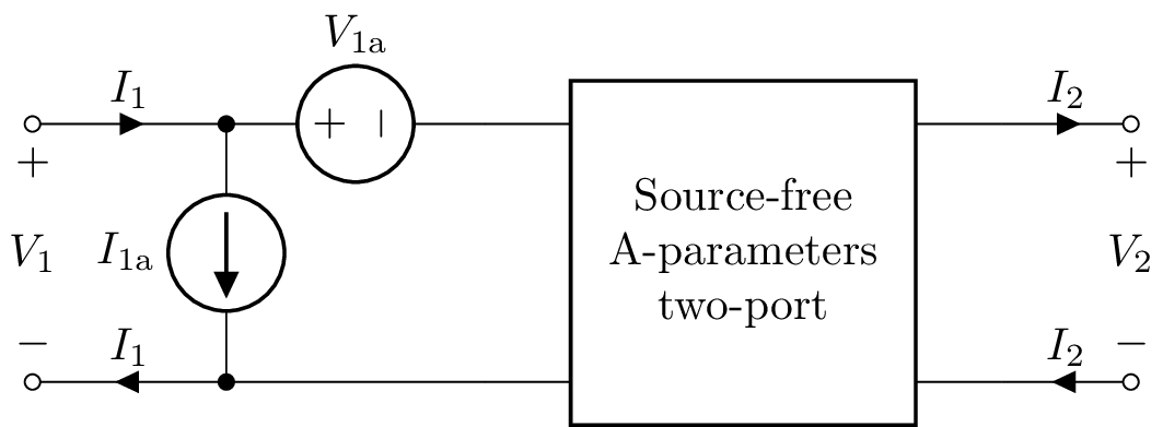
A-parameter two-port
An A-parameter two-port model is created with:
>>> n = TPA(A11, A12, A21, A22, V1a, I1a)
By default V1a=0 and I1a=0.
There are optional keyword arguments (kwargs) to specify schematic attributes, for example:
>>> n = TP(l='Two-port', fill='blue')
B-parameter two-port
A B-parameter two-port model is created with:
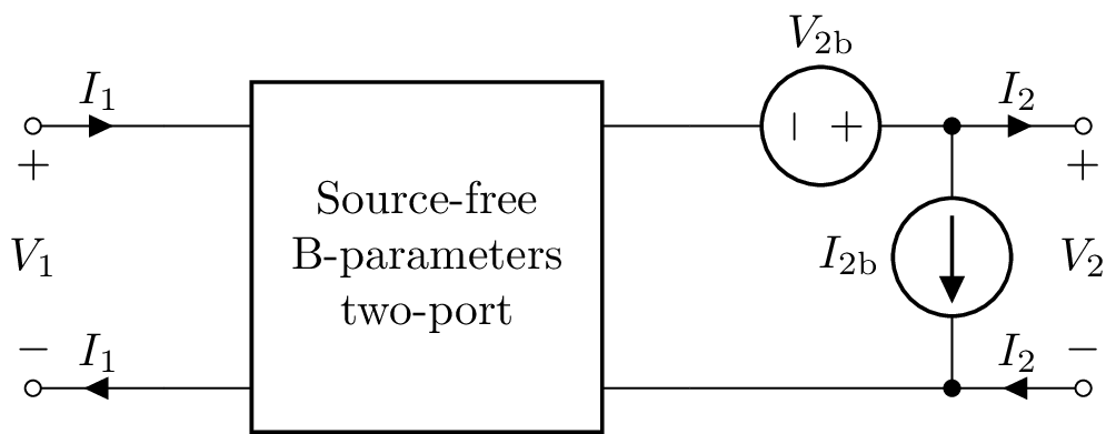
>>> n = TPB(B11, B12, B21, B22, V2b, I2b)
By default V2b=0 and I2b=0.
G-parameter two-port
A G-parameter two-port model is created with:
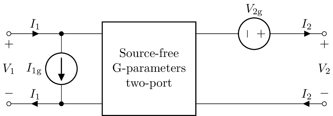
>>> n = TPG(G11, G12, G21, G22, I1g, V2g)
By default I1g=0 and V2g=0.
H-parameter two-port
A H-parameter two-port model is created with:
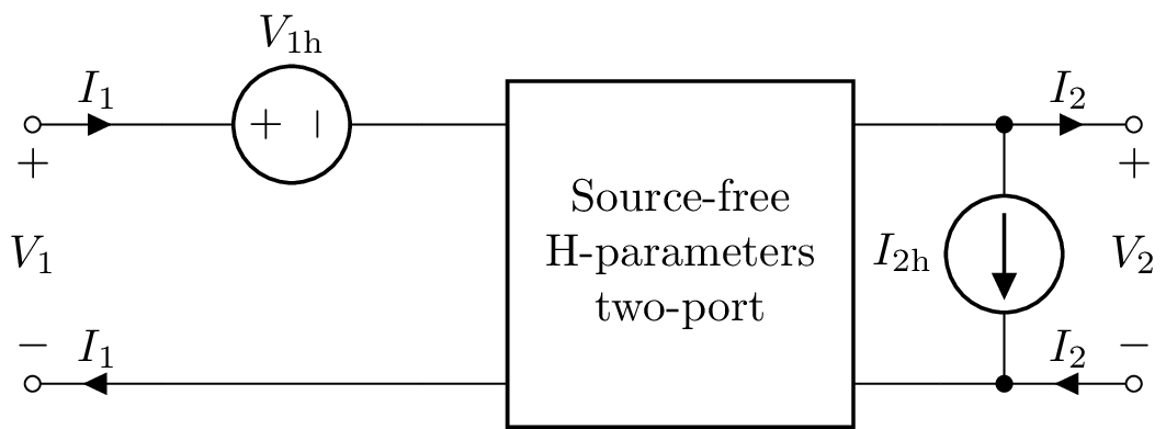
>>> n = TPH(H11, H12, H21, H22, V1h, I2h)
By default V1h=0 and I2h=0.
Y-parameter two-port
A Y-parameter two-port model is created with:
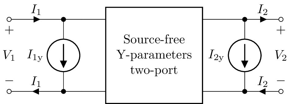
>>> n = TPY(Y11, Y12, Y21, Y22, I1y, I2y)
By default I1y=0 and I2y=0.
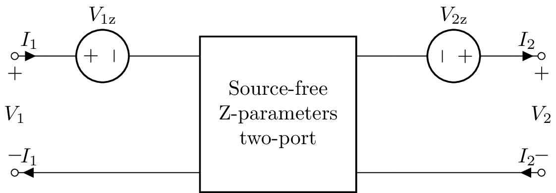
Z-parameter two-port
A Z-parameter two-port model is created with:
>>> n = TPZ(Z11, Z12, Z21, Z22, V1z, V2z)
By default V1z=0 and V2z=0.
Shunt two-port
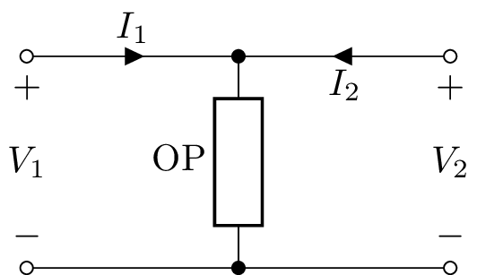
A shunt two-port has a single one-port argument, Shunt(OP), for example:
>>> n = Shunt(R('R1'))
The A-parameters are:
>>> n.Amodel.params
⎡1   0⎤
⎢     ⎥
⎢1    ⎥
⎢──  1⎥
⎣R₁   ⎦
The Y-parameters do not exist for a Shunt two-port.
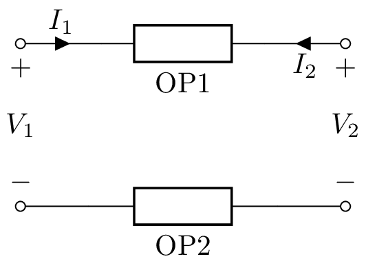
Series two-port
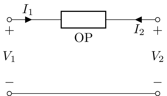
A series two-port has a single one-port argument, Series(OP), for example:
>>> n = Series(L('L1'))
The A-parameters can be found using:
>>> n.Amodel.params
⎡1  L₁⋅s⎤
⎢       ⎥
⎣0   1  ⎦
The Z-parameters do not exist for a Series two-port.
Series-pair two-port
A series-pair two-port is a balanced version of a series two-port. It has two one-port arguments, SeriesPair(OP1, OP2), for example:
>>> n = SeriesPair(L('L1/2'), L('L1/2'))
The A-parameters can be found using:
>>> n.Amodel.params
⎡1  L₁⋅s⎤
⎢       ⎥
⎣0   1  ⎦
Electrically, SeriesPair is the same as Series chained to another Series two-port. The Z-parameters do not exist for a SeriesPair two-port; the same as for a Series two-port.
L-section two-port
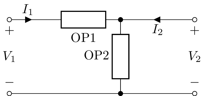
An L-section two-port has two one-port arguments, LSection(OP1, OP2), for example:
>>> n = LSection(L('L1'), R('R1'))
This is equivalent to chaining a shunt two-port to a series two-port:
>>> n = Series(L('L1').chain(Shunt(R('R1')))
For a balanced version of PiSection use CSection.
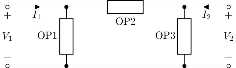
T-section two-port
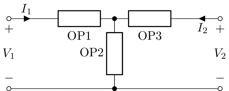
A T-section (also known as a Y-section) two-port has three one-port arguments, TSection(OP1, OP2, OP3), for example:
>>> n = TSection(L('L1'), R('R1'), C('C1'))
For a balanced version of PiSection use HSection.
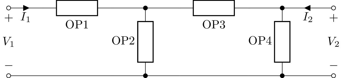
Pi-section two-port
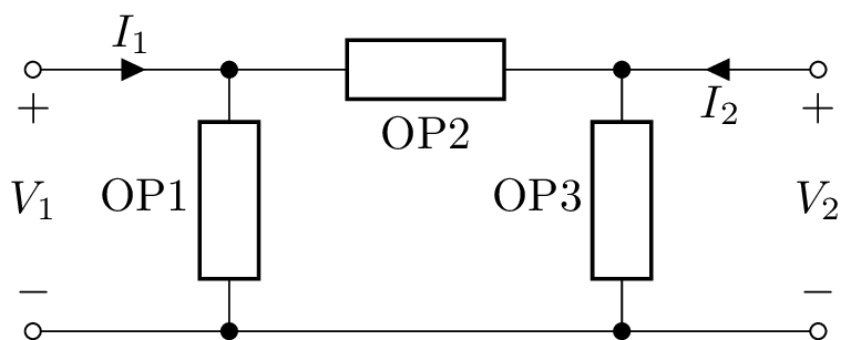
A pi-section two-port has three one-port arguments, PiSection(OP1, OP2, OP3), for example:
>>> n = PiSection(L('L1'), R('R1'), C('C1'))
For a balanced version of PiSection use BoxSection.
Ladder two-port
A ladder two-port has one or more one-port arguments, Ladder(OP1, OP2, OP3, …). The first argument is considered a Series element, the second is considered a Shunt element, the third is considered a Series element and so on. For example:
>>> n = Ladder(L('L1'), R('R1'), C('C1'))
The LadderAlt class is similar to Ladder but the alternating sequence of elements starts with a Shunt element. For example:
Transmission lines
There are three transmission line two-port classes: TransmissionLine, LosslessTransmissionLine and GeneralTransmissionLine. Here’s an example of use:
>>> a = GeneralTransmissionLine()
>>> a.equation()
       ⎡ cosh(l⋅γ(s))   -Z₀(s)⋅sinh(l⋅γ(s))⎤
⎡V₂⎤   ⎢                                   ⎥ ⎡V₁ ⎤
⎢  ⎥ = ⎢-sinh(l⋅γ(s))                      ⎥⋅⎢   ⎥
⎣I₂⎦   ⎢──────────────     cosh(l⋅γ(s))    ⎥ ⎣-I₁⎦
       ⎣    Z₀(s)                          ⎦
Here \(Z_0\) is the characteristic impedance, \(\gamma\) is the propagation constant, and \(l\) is the transmission line length. These can be specified when GeneralTransmissionLine is constructed.
The input impedance to the transmission line can be found from the Z11 parameter:
>>> a.Z11
    Z₀
─────────
tanh(γ⋅l)
List of two-ports
Shunt
Series
SeriesAlt
SeriesPair
LSection
LSectionAlt
TSection
PiSection
CSection
HSection
BoxSection
GenericTwoPort
IdealTransformer
IdealGyrator
VoltageFollower
VoltageAmplifier
IdealVoltageAmplifier
IdealDelay
IdealVoltageDifferentiator
IdealVoltageIntegrator
CurrentFollower
IdealCurrentAmplifier
IdealCurrentDifferentiator
IdealCurrentIntegrator
OpampInverter
OpampIntegrator
OpampDifferentiator
TwinTSection
BridgedTSection
Ladder
LadderAlt
GeneralTransmissionLine
LosslessTransmissionLine
TransmissionLine
TPA
TPB
TPG
TPH
TPY
TPZ
Two-port network attributes
Here are some of the two-port network attributes:
is_bilateral: True if the two-port is bilateral
is_buffered: True if the two-port is buffered, i.e., any load on the output has no affect on the input
is_reciprocal: True if the two-port is reciprocal
is_series: True if the two-port is a series network
is_shunt: True if the two-port is a shunt network
is_symmetrical: True if the two-port is symmetrical
Voc: voltage vector with both ports open-circuit
V1oc: open-circuit input voltage
V2oc: open-circuit output voltage
Isc: current vector with both ports short-circuit
I1sc: short-circuit input current
I2sc: short-circuit output current
Zoc: impedance vector with both ports open-circuit
Z1oc: input impedance with output port open-circuit
Z2oc: output impedance with input port open-circuit
Ysc: admittance vector with both ports short-circuit
Y1sc: input admittance with output port short-circuit
Y2sc: output admittance with input port short-circuit
Amodel: the equivalent A-parameters model (ABCD)
Bmodel: the equivalent B-parameters model (inverse ABCD)
Gmodel: the equivalent G-parameters model (inverse hybrid / parallel-series)
Hmodel: the equivalent H-parameters model (hybrid / series-parallel)
Ymodel: the equivalent Y-parameters model (admittance)
Zmodel: the equivalent Z-parameters model (impedance)
Aparams: the A-parameters (ABCD)
Bparams: the A-parameters (inverse ABCD)
Gparams: the G-parameters (inverse hybrid / parallel-series)
Hparams: the H-parameters (hybrid / series-parallel)
Sparams: the S-parameters (scattering)
Tparams: the T-parameters (scattering transmission)
Yparams: the Y-parameters (admittance)
Zparams: the Z-parameters (impedance)
params: the 2x2 matrix of parameters
sources: the 2x1 vector of sources
The individual elements of a parameter matrix for a two-port n can be accessed using n.A11, n.S21, n.Z22 etc.
Two-port network methods
Here are some of the two-port network methods:
chain(TP): chain (cascade) two two-port networks together
series(TP): combine two two-port networks in series
parallel(TP): combine two two-port networks in parallel
hybrid(TP): combine two two-port networks in series-parallel
inverse_hybrid(TP): combine two two-port networks in parallel-series
bridge(OP): bridge a two-port network with a one-port network
load(OP): apply a one-port network load and return a one-port network
source(OP): apply a one-port network source and return a one-port network
draw(): draw a two-port network
circuit(): convert a two-port network to a Circuit object
equation(): return the system of equations in matrix form
Two-port combinations
Two-port networks can be combined in series, parallel, series at the input with parallel at the output (hybrid), parallel at the input with series at the output (inverse hybrid), but the most common is the chain or cascade. This connects the output of the first two-port to the input of the second two-port.
For example, an L section can be created by chaining a shunt to a series one-port:
>>> from lcapy import *
>>> n = Series(R('R_1')).chain(Shunt(R('R_2')))
>>> n.Vtransfer
R_2/(R_1 + R_2)
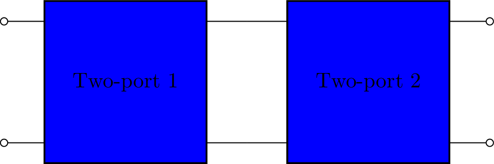
Chain
>>> from lcapy import TP
>>> tp1 = TP(l='Two-port 1', fill='blue')
>>> tp2 = TP(l='Two-port 2', fill='blue')
>>> tp = tp1.chain(tp2)
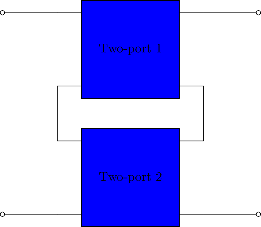
Parallel
>>> from lcapy import TP
>>> tp1 = TP(l='Two-port 1', fill='blue')
>>> tp2 = TP(l='Two-port 2', fill='blue')
>>> tp = tp1.parallel(tp2)
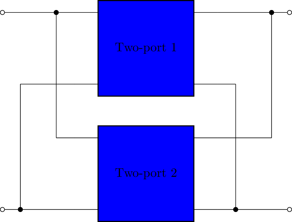
Series
Warning, a series combination of two-ports can break the port condition.
>>> from lcapy import TP
>>> tp1 = TP(l='Two-port 1', fill='blue')
>>> tp2 = TP(l='Two-port 2', fill='blue')
>>> tp = tp1.series(tp2)
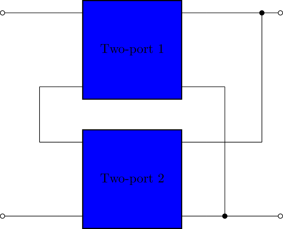
Hybrid (series-parallel)
>>> from lcapy import TP
>>> tp1 = TP(l='Two-port 1', fill='blue')
>>> tp2 = TP(l='Two-port 2', fill='blue')
>>> tp = tp1.hybrid(tp2)
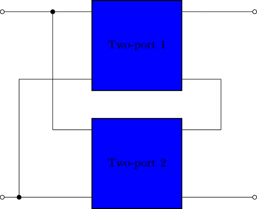
Inverse hybrid (parallel-series)
>>> from lcapy import TP
>>> tp1 = TP(l='Two-port 1', fill='blue')
>>> tp2 = TP(l='Two-port 2', fill='blue')
>>> tp = tp1.hybrid(tp2)
Two-port network models
Lcapy describes two-port networks in the Laplace domain using A, B, G, H, S, T, Y, and Z matrices. Note, for some network configurations some of these matrices can be singular.
Each model can be converted to the other parameterisations, for example:
>>> A = TPA()
>>> TPA.params
>>> A.Zmodel.params
The elements of the parameter matrix can be accessed by name, for example:
>>> A.S11
Note, in this example, the A-parameters are converted to S-parameters.
A-parameters (ABCD)
The A matrix is the inverse of the B matrix.
B-parameters (inverse ABCD)
The B matrix is the inverse of the A matrix.
G-parameters (inverse hybrid)
The G matrix is the inverse of the H matrix.
H-parameters (hybrid)
The H matrix is the inverse of the G matrix.
S-parameters (scattering)
T-parameters (scattering transfer)
Y-parameters (admittance)
The Y matrix is the inverse of the Z matrix.
Z-parameters (impedance)
The Z matrix is the inverse of the Y matrix.