Advanced circuit analysis
Transmission lines
A lossless transmission line with characteristic impedance \(Z_0\), speed of propagation \(c\), and length \(l\) driven by a step voltage \(V_s\) through a resistance \(R_s\), and loaded with a resistance \(R_l\) can be defined as:
Vs 1 0 step; down
Rs 1 2a; right
W 2a 2; right=0.5
TL 3 0_3 2 0_2 lossless; right, l=Z_0
W 3 4; right=0.5
Rl 4 0_4; down
W 0_3 0_4; right
W 0 0_2; right
P2 3 0_3; down, v=V_2
P1 2 0_2; down, v_=V_1
; draw_nodes=connections, label_nodes=none
Lcapy can draw this using:
>>> from lcapy import Circuit, s, t
>>> a = Circuit('txline1.sch')
>>> a.draw()

The driving-point impedance looking into the start of the transmission line is:
>>> a.P1.dpZ
                   ⎛       ⎛l⋅s⎞          ⎛l⋅s⎞⎞
             Rₛ⋅Z₀⋅⎜Rₗ⋅cosh⎜───⎟ + Z₀⋅sinh⎜───⎟⎟
                   ⎝       ⎝ c ⎠          ⎝ c ⎠⎠
───────────────────────────────────────────────────────────────────
          ⎛l⋅s⎞             ⎛l⋅s⎞             ⎛l⋅s⎞     2     ⎛l⋅s⎞
Rₗ⋅Rₛ⋅sinh⎜───⎟ + Rₗ⋅Z₀⋅cosh⎜───⎟ + Rₛ⋅Z₀⋅cosh⎜───⎟ + Z₀ ⋅sinh⎜───⎟
          ⎝ c ⎠             ⎝ c ⎠             ⎝ c ⎠           ⎝ c ⎠
Similarly, the driving-point impedance looking into the end of the transmission line is:
>>> a.P2.dpZ
                      ⎛       ⎛l⋅s⎞          ⎛l⋅s⎞⎞
                Rₗ⋅Z₀⋅⎜Rₛ⋅cosh⎜───⎟ + Z₀⋅sinh⎜───⎟⎟
                      ⎝       ⎝ c ⎠          ⎝ c ⎠⎠
───────────────────────────────────────────────────────────────────
          ⎛l⋅s⎞             ⎛l⋅s⎞             ⎛l⋅s⎞     2     ⎛l⋅s⎞
Rₗ⋅Rₛ⋅sinh⎜───⎟ + Rₗ⋅Z₀⋅cosh⎜───⎟ + Rₛ⋅Z₀⋅cosh⎜───⎟ + Z₀ ⋅sinh⎜───⎟
          ⎝ c ⎠             ⎝ c ⎠             ⎝ c ⎠           ⎝ c ⎠
The Laplace domain voltage across the input of the transmission line is
>>> a.P1.V(s)
                        ⎛       ⎛l⋅s⎞          ⎛l⋅s⎞⎞
                  Vₛ⋅Z₀⋅⎜Rₗ⋅cosh⎜───⎟ + Z₀⋅sinh⎜───⎟⎟
                        ⎝       ⎝ c ⎠          ⎝ c ⎠⎠
───────────────────────────────────────────────────────────────────────
  ⎛          ⎛l⋅s⎞             ⎛l⋅s⎞             ⎛l⋅s⎞     2     ⎛l⋅s⎞⎞
s⋅⎜Rₗ⋅Rₛ⋅sinh⎜───⎟ + Rₗ⋅Z₀⋅cosh⎜───⎟ + Rₛ⋅Z₀⋅cosh⎜───⎟ + Z₀ ⋅sinh⎜───⎟⎟
  ⎝          ⎝ c ⎠             ⎝ c ⎠             ⎝ c ⎠           ⎝ c ⎠⎠
and the Laplace domain voltage across the output of the transmission line is
>>> a.P2.V(s)
                               Rₗ⋅Vₛ⋅Z₀
───────────────────────────────────────────────────────────────────────
  ⎛          ⎛l⋅s⎞             ⎛l⋅s⎞             ⎛l⋅s⎞     2     ⎛l⋅s⎞⎞
s⋅⎜Rₗ⋅Rₛ⋅sinh⎜───⎟ + Rₗ⋅Z₀⋅cosh⎜───⎟ + Rₛ⋅Z₀⋅cosh⎜───⎟ + Z₀ ⋅sinh⎜───⎟⎟
  ⎝          ⎝ c ⎠             ⎝ c ⎠             ⎝ c ⎠           ⎝ c ⎠⎠
Since the transmission line is lossless, the transient response has an infinite number of reflections. At the end of the transmission line
>>> a.P2.V(t)
           ∞
         _____
         ╲
          ╲                                 m
           ╲   ⎛                          2⎞
            ╲  ⎜Rₗ⋅Rₛ - Rₗ⋅Z₀ - Rₛ⋅Z₀ + Z₀ ⎟   ⎛    l⋅(2⋅m + 1)⎞
Rₗ⋅Vₛ⋅Z₀⋅   ╱  ⎜───────────────────────────⎟ ⋅u⎜t - ───────────⎟
           ╱   ⎜                          2⎟   ⎝         c     ⎠
          ╱    ⎝Rₗ⋅Rₛ + Rₗ⋅Z₀ + Rₛ⋅Z₀ + Z₀ ⎠
         ╱
         ‾‾‾‾‾
        m = 0
────────────────────────────────────────────────────────────────
                                            2
                  Rₗ⋅Rₛ + Rₗ⋅Z₀ + Rₛ⋅Z₀ + Z₀
The transient response at the start of the transmission line can be found in a similar way but is too long to show here.
If the transmission line is terminated at the load with its characteristic impedance:
>>> b = a.subs({'Rl':'Z0'})
>>> b.P1.V(s)
⎛ Vₛ⋅Z₀ ⎞
⎜───────⎟
⎝Rₛ + Z₀⎠
─────────
    s
>>> b.P1.V(t)
Vₛ⋅Z₀⋅u(t)
──────────
 Rₛ + Z₀
>>> b.P2.V(s)
                               Vₛ⋅Z₀
─────────────────────────────────────────────────────────────
  ⎛       ⎛l⋅s⎞          ⎛l⋅s⎞          ⎛l⋅s⎞          ⎛l⋅s⎞⎞
s⋅⎜Rₛ⋅sinh⎜───⎟ + Rₛ⋅cosh⎜───⎟ + Z₀⋅sinh⎜───⎟ + Z₀⋅cosh⎜───⎟⎟
  ⎝       ⎝ c ⎠          ⎝ c ⎠          ⎝ c ⎠          ⎝ c ⎠⎠
>>> b.P2.V(t)
       ⎛    l⎞
Vₛ⋅Z₀⋅u⎜t - ─⎟
       ⎝    c⎠
──────────────
   Rₛ + Z₀
If the transmission line is terminated at the source with its characteristic impedance:
>>> c = a.subs({'Rs':'Z0'})
>>> c.P1.V(s)
                  ⎛       ⎛l⋅s⎞          ⎛l⋅s⎞⎞
               Vₛ⋅⎜Rₗ⋅cosh⎜───⎟ + Z₀⋅sinh⎜───⎟⎟
                  ⎝       ⎝ c ⎠          ⎝ c ⎠⎠
─────────────────────────────────────────────────────────────
  ⎛       ⎛l⋅s⎞          ⎛l⋅s⎞          ⎛l⋅s⎞          ⎛l⋅s⎞⎞
s⋅⎜Rₗ⋅sinh⎜───⎟ + Rₗ⋅cosh⎜───⎟ + Z₀⋅sinh⎜───⎟ + Z₀⋅cosh⎜───⎟⎟
  ⎝       ⎝ c ⎠          ⎝ c ⎠          ⎝ c ⎠          ⎝ c ⎠⎠
>>> c.P1.V(t)
   ⎛    2     2⎞ ⎛u(t)    ⎛    2⋅l⋅m⎞⎞
Vₛ⋅⎝- Rₗ  + Z₀ ⎠⋅⎜──── + u⎜t - ─────⎟⎟
                 ⎝ 2      ⎝      c  ⎠⎠
──────────────────────────────────────
     -Rₗ⋅(Rₗ + Z₀) + Z₀⋅(Rₗ + Z₀)
>>> c.P1.V(t).simplify()
   ⎛u(t)    ⎛    2⋅l⋅m⎞⎞
Vₛ⋅⎜──── + u⎜t - ─────⎟⎟
   ⎝ 2      ⎝      c  ⎠⎠
>>> c.P2.V(s)
                            Rₗ⋅Vₛ
─────────────────────────────────────────────────────────────
  ⎛       ⎛l⋅s⎞          ⎛l⋅s⎞          ⎛l⋅s⎞          ⎛l⋅s⎞⎞
s⋅⎜Rₗ⋅sinh⎜───⎟ + Rₗ⋅cosh⎜───⎟ + Z₀⋅sinh⎜───⎟ + Z₀⋅cosh⎜───⎟⎟
  ⎝       ⎝ c ⎠          ⎝ c ⎠          ⎝ c ⎠          ⎝ c ⎠⎠
>>> c.P2.V(t)
       ⎛    l⎞
Rₗ⋅Vₛ⋅u⎜t - ─⎟
       ⎝    c⎠
──────────────
   Rₗ + Z₀
In this case, there is a single reflection.
Piezoelectric transducers
A piezoelectric transducer can be modelled with the KLM model. This can be described with the following netlist:
Cable1; right=2, kind=coax, l=Z_0
W 1 Cable1.in; right=0.5, i=U_b
W Cable1.out 2; right=0.5
W Cable1.ignd 1_0; down=0.5
W 14_0 1_0; right=0.5
Pb 1 14_0; down, v_=F_b

Cable2; right=2, kind=coax, l=Z_0
W 2 Cable2.in; right=0.5
W Cable2.out 3; right=0.5, i<=U_f
W Cable2.ognd 3_0; down=0.5
W 3_0 13_0; right=0.5
Pf 3 13_0; down, v^=F_f

W 2 4; down=1.5
W Cable2.ignd 5; down=0.1
W Cable1.ognd 6; down=0.1
W 6 5; right

TF1 4 7 8 9 phi; right
W 7 10; right=0.5
W 5 10; down

Pe 11 0; down, v_=V
C0 11 12; right, i>^=I
Z 12 8 {j * X_1}; right
W 0 9; right

W 9 7; right, ignore

; draw_nodes=connections, label_nodes=none, label_ids=none
Lcapy can draw this using:
>>> from lcapy import Circuit, s, t
>>> a = Circuit('KLM2.sch')
>>> a.draw()
In the Laplace domain, the transformer coupling ratio is
\(\phi = \frac{s Z_0}{2 h} \frac{1}{\sinh\left(\frac{s d}{2 c}\right)}\),
the impedance of X1 is
\(X_1 = \frac{j h^2}{s^2 Z_0} \sinh\left(\frac{s d}{c}\right)\),
and
\(C_0 = \frac{\epsilon^{S} A}{d}\),
where \(Z_0\) is the characteristic impedance of the piezoelectric crystal, \(h\) is the pressure constant of the crystal, \(d\) is the thickness of the crystal, and \(\epsilon^{S}\) is the clamped (zero strain,high frequency) permittivity of the crystal.
The model has three ports: an electrical port, a back mechanical port, and a front mechanical port.
The above netlist is not suitable for simulation since the transmission lines are represented with cables; Lcapy treats them as ideal wires. Instead transmission line components are required as in the following netlist:
Pb 1 0_1; down, v_=F_b
TLb 2 6 1 0_1 Z_0 {s / c} {d / 2}; right

Pf 3 0_3; down, v^=F_f
TLf 3 0_3 15 5 Z_0 {s / c} {d / 2}; right

W 2 15; right=0.5
W 2 4; down=1.5
W 6 5; right=0.5

TF1 4 7 8 9 phi; right
W 9 7; right=0.5, dashed
W 7 10; right=0.5
W 5 10; down

Pe 11 0; down, v_=V
C0 11 12; right, i>^=I
Z 12 8 {j * X_1}; right
W 0 9; right

W 9 7; right, ignore

; draw_nodes=connections, label_nodes=none, label_ids=none
This is drawn as
Let’s consider finding the ratio of the force across the front mechanical port given an applied voltage across the electrical port with the back mechanical port free. With the back port free, there is no force across it. This can be asserted by applying a short-circuit across Pb. For example,
>>> from lcapy import Circuit
>>> a = Circuit('KLM-demo.sch')
>>> a.short_circuit('Pb')
The ratio of the mechanical force to an applied voltage can be found using the voltage_gain() method of the circuit:
>>> H = a.voltage_gain('Pe', 'Pf')
                                                  ⎛d⋅s⎞
                               -2⋅ⅉ⋅C₀⋅Z₀⋅φ⋅s⋅sinh⎜───⎟
                                                  ⎝2⋅c⎠
───────────────────────────────────────────────────────────────────────────────────────
         2       2⎛d⋅s⎞            2       ⎛            ⎛d⋅s⎞      2     2⎛d⋅s⎞      2⎞
4⋅C₀⋅X₁⋅φ ⋅s⋅sinh ⎜───⎟ + 2⋅C₀⋅X₁⋅φ ⋅s - ⅉ⋅⎜C₀⋅Z₀⋅s⋅sinh⎜───⎟ + 4⋅φ ⋅sinh ⎜───⎟ + 2⋅φ ⎟
                  ⎝2⋅c⎠                    ⎝            ⎝ c ⎠             ⎝2⋅c⎠       ⎠
The frequency response can be found by substituting \(j 2 \pi f\) for \(s\).
Transformers
The Lcapy TF component represents an ideal transformer. Indeed it operates at DC!
To model a real transformer, a pair of magnetically coupled inductors is required. The coupling is specified by the K component. This has three arguments: the names of two inductors and a coupling coefficient k. The mutual inductance of the two inductors is:
\(M = k \sqrt{L_1 L_2}\).
The inductances are related by the number of turns by:
\(L = \frac{N}{\mathcal{R}}\)
where \(\mathcal{R}\) is the reluctance. If both inductors have a similar reluctance:
\(\frac{N_1}{N_2} = \sqrt{\frac{L_1}{L_2}}\)
Note, this is an approximation and depends on the inductor geometry and the cores.
The equations for a pair of coupled inductors is
\(v_1(t) = L_1 \frac{\mathrm{d}}{\mathrm{d} t} i_1(t) + M \frac{\mathrm{d}}{\mathrm{d} t} i_2(t)\)
\(v_2(t) = M \frac{\mathrm{d}}{\mathrm{d} t} i_1(t) + L_2 \frac{\mathrm{d}}{\mathrm{d} t} i_2(t)\)
where \(M\) is the mutual inductance. This circuit can be described in Lcapy with the netlist:
W 1 1a; right, i=i_1
L1 1a 2a; down
W 2 2a; right
K L1 L2 k; right=1.2
W 3 3a; left, i=i_2
L2 3a 4a; down
W 4a 4; right
P1 1 2; down, v_=v_1
P2 3 4; down, v^=v_2
;label_nodes=False, draw_nodes=connections
However, it cannot be analysed since the secondary has no reference to the primary. One approach is to couple the primary and secondary circuits with a resistor and consider the result in the limit as the resistor is made infinite. There is no problem if the primary and secondary share a common ground as in the figure below:
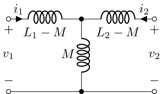
A transformer with a common ground for the primary and secondary can be represented by a tee-model without having to use a coupling K component. In this case, the voltages can be expressed in terms of the currents using:
\(v_1(t) = \left(L_1 - M\right) \frac{\mathrm{d}}{\mathrm{d} t} i_1(t) + M \frac{\mathrm{d}}{\mathrm{d} t} \left(i_1 - i_2(t)\right)\)
\(v_2(t) = M \frac{\mathrm{d}}{\mathrm{d} t} \left(i_1(t) - i_2(t)\right) + \left(L_2 - M\right) \frac{\mathrm{d}}{\mathrm{d} t} i_2(t)\)
Here \(L_1\) is the primary magnetising inductance, \(L_2\) is the secondary magnetising inductance, \(L_1 - M\) is the primary leakage inductance, and \(L_2 - M\) is the secondary leakage inductance. These equations correspond to the following circuit:
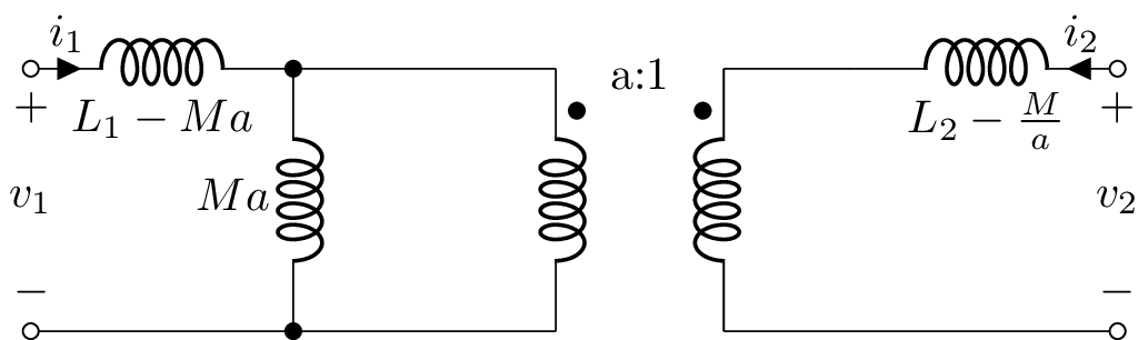
Sometimes a transformer is modelled around an ideal transformer with turns ratio \(a = N_1 / N_2\) as per the following circuit:
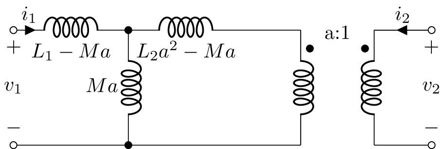
Sometimes the secondary leakage inductance is referred to the primary:
Non-linear analysis using state-space
Let’s consider the step-response of a CMOS device switching from low to high. In the circuit below, the capacitance Cl denotes a capacitive load, say the input of another CMOS device, Rs is a series resistance, say to control the rise-time’, and Vt and Rt comprise a Thevenin load, say due to a pull-up resistor.
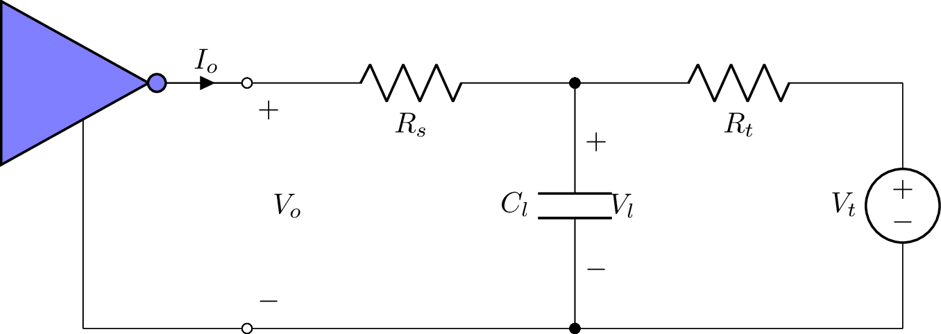
Using an IBIS output model to model the parasitic components, the equivalent circuit is:
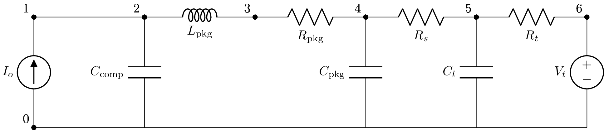
In this model, the CMOS output is modelled as a voltage dependent current-source, \(I_o(V_o)\). The netlist is:
Io 1 0; down
W 1 2; right=1.5
Ccomp 2 0_2; down
Lpkg 2 3; right=1.5
Rpkg 3 4; right=1.5
Cpkg 4 0_4; down
W 0 0_2; right
W 0_2 0_4; right
Rs 4 5; right=1.5
Cl 5 0_5; down
W 0_4 0_5; right
Rt 5 6; right=1.5
Vt 6 0_6; down=1.5
W 0_5 0_6; right
Using this netlist, a state-space model can be created:
>>> from lcapy import Circuit
>>> cct = Circuit('cmos_ibis_R_series_C_load_thevenin.sch')
>>> ss = cct.state_space(node_voltages=(1, 5), branch_currents=())
Here the outputs are the node voltages 1 and 5 corresponding to the output voltage \(V_o\) and the load voltage \(V_l\) across Cl. The state vector is
>>> ss.x
⎡i_Lpkg(t) ⎤
⎢          ⎥
⎢v_Ccomp(t)⎥
⎢          ⎥
⎢v_Cpkg(t) ⎥
⎢          ⎥
⎣ v_Cl(t)  ⎦
the input vector is
>>> ss.u
⎡Vₜ⎤
⎢  ⎥
⎣Iₒ⎦
the output vector is
>>> ss.y
⎡v₁(t)⎤
⎢     ⎥
⎣v₅(t)⎦
and the system matrices are
>>> ss.A
⎡-R_pkg     1      -1                     ⎤
⎢───────  ─────   ─────           0       ⎥
⎢ L_pkg   L_pkg   L_pkg                   ⎥
⎢                                         ⎥
⎢ -1                                      ⎥
⎢──────     0       0             0       ⎥
⎢C_comp                                   ⎥
⎢                                         ⎥
⎢   1              -1            1        ⎥
⎢ ─────     0    ────────     ────────    ⎥
⎢ C_pkg          C_pkg⋅Rₛ     C_pkg⋅Rₛ    ⎥
⎢                                         ⎥
⎢                   1          1       1  ⎥
⎢   0       0     ─────    - ───── - ─────⎥
⎣                 Cₗ⋅Rₛ      Cₗ⋅Rₜ   Cₗ⋅Rₛ⎦
>>> ss.B
⎡  0      0   ⎤
⎢             ⎥
⎢         1   ⎥
⎢  0    ──────⎥
⎢       C_comp⎥
⎢             ⎥
⎢  0      0   ⎥
⎢             ⎥
⎢  1          ⎥
⎢─────    0   ⎥
⎣Cₗ⋅Rₜ        ⎦
>>> ss.C
⎡0  1  0  0⎤
⎢          ⎥
⎣0  0  0  1⎦
>>> ss.D
⎡0  0⎤
⎢    ⎥
⎣0  0⎦
Since the CMOS device is non-linear, there is no analytic solution and a numerical solution is required. This can be achieved using the SciPy solve_ivp function.
>>> A = array(((-Rpkg / Lpkg, 1 / Lpkg, -1 / Lpkg, 0),
               (-1 / Ccomp, 0, 0, 0),
               (1 / Cpkg, 0, -1 / (Cpkg * Rs), 1 / (Cpkg * Rs)),
               (0, 0, 1 / (CL * Rs), -1 / (CL * Rs) - 1 / (CL * Rt))))
>>> B = array(((0, 0),
               (0, 1 / Ccomp),
               (0, 0),
               (1 / (CL * Rt), 0)))
>>> C = array(((0, 1, 0, 0),
               (0, 0, 0, 1)))
>>> D = array(((0, 0),
               (0, 0)))
>>>
>>> def func(t, x):
>>>    y = dot(C, x)
>>>    Vo = y[0]
>>>    Vl = y[1]
>>>    Io = lookup_Io(Vo)
>>>    u = array((Vt, Io))
>>>    xdot = dot(A, x) + dot(B, u)
>>>    return xdot
>>>
>>> ret = solve_ivp(func, [t[0], t[-1]], [0, 0, 0, 0], t_eval=t)
>>>
>>> Vl = ret.y[3].squeeze()
In this snippet of code, the line lookup_Io(Vo) determines the output current for a specific output voltage, say by interpolating a lookup table.
Note, solve_ivp can choose a poor initial step for this circuit. A work-around is to scale the capacitances, inductances, and time.