Troubleshooting
Most Lcapy problems are due to symbol assumptions and approximation of floating-point values as rational numbers. If you want to report a bug, see Issue reporting. If you would like to debug the problem, see Debugging.

Common problems
Variable names
SymPy does not allow symbol names that are Python keywords. For example, expr(‘is(t)’) fails. A workaround is to use an underscore in the name, for example, expr(‘i_s(t)’).
Predefined symbols
A number of symbols are predefined by Lcapy and Sympy including: - delta for Dirac delta - j for imaginary operator - u for unit step (Heaviside function) - H for Heaviside function - I for imaginary operator - jf, jw, `f, k, n, s, t, w, z for domain variables
Floating point values
Floating point numbers are an extremely poor approximation of real numbers; rational numbers are slightly better and this is what Lcapy uses to help with expression simplification. However, there is a loss of precision when converting a floating-point number to a rational number. For example, consider:
>>> 2 / 3
3333333333333333
────────────────
5000000000000000
In this case, Python evaluates 2 / 3 as a floating-point number which is then converted to a rational number. Unfortunately, this is not quite the same as 2 / 3. The approximation can be avoided by bypassing the conversion of 2 / 3 to 0.666666666666, say by using:
>>> expr('2 / 3')
2/3
Another approach is to use:
>>> one * 2 / 3
2/3
Here one is a SymPy object representing the number 1.
Equality
For equality Lcapy requires expressions to have the same domain and quantity. There are some exceptions to the domain requirement when comparing constants. However, a voltage expression is not equal to a current expression. For example:
>>> V = voltage(7)
>>> I = current(7)
>>> V == I
False
>>> V.quantity
'voltage'
>>> I.quantity
'current'
The quantity can be removed using the as_expr() method. For example:
>>> V.as_expr() == I.as_expr()
True
Even when expressions have the same domain and quantity a test for equality can fail. This is because SymPy comparison uses structural equality, see https://docs.sympy.org/latest/gotchas.html
- One way to test for equality is to subtract the expressions, simplify, and test for 0. For example,
>>> (x - y).simplify() == 0
However, there is no gaurantee that SymPy simplification will return 0 for equal expressions.
Symbol aliases
SymPy treats symbols with different assumptions as different symbols even if they have the same name. To reduce this confusion, Lcapy assumes that symbol names are not aliased. It achieves this by maintaining a dictionary of defined symbols for each circuit. However, it is unaware of symbols created by SymPy.
Here’s an example of how to access the symbols:
>>> from lcapy import symbol
>>> x = symbol('x')
>>> state.context.symbols
{'s': s,
't': t,
'f': f,
'omega': omega,
'omega_0': omega_0,
'tau': tau,
'x': x}
This shows the pre-defined symbols and the newly defined symbol. Each directory entry is a SymPy symbol.
Symbol assumptions
There can be difficulties with symbol assumptions when working with SymPy. By default SymPy creates symbols with few assumptions, for example,
>>> from sympy import Symbol
>>> R1 = Symbol('R')
>>> R1.assumptions0
{'commutative': True}
On the other hand, by default, Lcapy assumes that symbols are positive (unless explicitly defined otherwise). For example,
>>> from lcapy import symbol
>>> R2 = symbol('R')
>>> R2.assumptions0
{'commutative': True,
'complex': True,
'hermitian': True,
'imaginary': False,
'negative': False,
'nonnegative': True,
'nonpositive': False,
'nonzero': True,
'positive': True,
'real': True,
'zero': False}
Since R1 and R2 have different assumptions, SymPy considers them different symbols even though they are both defined with the same name R.
Note, every real symbol is also considered complex although with no imaginary part. The proper way to test assumptions is to use the attributes is_complex, is_real, etc. For example,
>>> t.is_real
True
>>> t.is_complex
False
Zero substitution
- Be careful with zero substitutions. For example, consider
>>> x = symbol('x')
>>> (x * (s + 1 / x)).subs(x, 0)
0
In general it is safer (but slower) to evaluate a limit at zero.
>>> x = symbol('x')
>>> (x * (s + 1 / x)).limit(x, 0)
1
Another approach is expand the expression to avoid the division:
>>> x = symbol('x')
>>> (x * (s + 1 / x)).expand().subs(x, 0)
1
Symbol confusion
j is an Lcapy symbol denoting the imaginary unit but 1j is a Python floating-point imaginary number.
pi is an Lcapy symbol denoting the transcendental number \(\pi\) but np.pi and math.pi is a floating-point number approximating \(\pi\).
MNA problems
Lcapy uses modified nodal analysis to determine the node voltages and branch currents. This requires inversion of a matrix but sometimes this matrix is singular. The common reasons for this are:
There are capacitors in series
A voltage source is short-circuited
A current source is open-circuited
The secondary of a transformer is floating (use a resistor or wire)
Nodes are unconnected (use cct.unconnected_nodes)
Simplification
Some expressions are difficult to simplify. Often this is due to a lack of symbol assumptions. Sometimes, it is better to use the simplify_terms() method to simplify each term separately.
Some simple circuits have gnarly solutions. For example, consider the network:

This has an admittance, Y(s):
          1
─────────────────────
            1
R₀ + ────────────────
                1
     C₁⋅s + ─────────
            L₁⋅s + R₁
which can be written in canonical form as:
     ⎛       2              ⎞
     ⎜C₁⋅L₁⋅s  + C₁⋅R₁⋅s + 1⎟
     ⎜──────────────────────⎟
     ⎝       C₁⋅L₁⋅R₀       ⎠
─────────────────────────────────
 2   s⋅(C₁⋅R₀⋅R₁ + L₁)   R₀ + R₁
s  + ───────────────── + ────────
          C₁⋅L₁⋅R₀       C₁⋅L₁⋅R₀
Despite this only being second, its inverse Laplace transform is too long to list here.
Computation speed
Lcapy can be slow for large problems due to the computational complexity of the algorithms (see Performance). If speed is important, it is better to substitute symbolic values with numerical values.
The results from slow computations are cached to improve the speed.
Some SymPy operations can take an unexpectedly long time, for example, limit(). With some versions of SymPy, symbolic matrix inversions are really slow.
Working with SymPy
Lcapy wraps many of SymPy’s methods but if you know how to use SymPy, you can extract the underlying SymPy expression using the sympy attribute of an Lcapy expression.
Most SymPy functions have Lcapy equivalents. You can mix Lcapy and Sympy expressions with the result being an Lcapy expression.
Printing
Importing Lcapy intercepts SymPy printing, thus the Sympy Functions pretty() and latex() work on Lcapy objects. Note, Lcapy objects have pretty() and latex() methods.
SymPy differences
SymPy defines \(sinc(x)\) as \(sin(x)/x\) but Lcapy (and NumPy) defines \(sinc(x)\) as \(sin(\pi x)/(\pi x)\), see Mathematical functions.
SymPy uses 0 for the lower limit of Laplace transforms, Lcapy uses \(0^{-}\), see Laplace transforms.
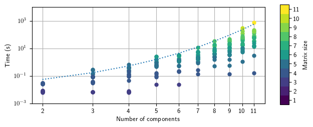
Performance
The performance of Lcapy depends on Sympy’s system of equations solver and root finding routines. The following figure shows the time taken to determine the open circuit voltage for twenty randomly generated networks with a specified number of components. Each network has a single voltage source and a number of resistors. The colour of the plot denotes the matrix size; this depends how the components are connected. In general, symbolic solving of a system of \(N\) equations in \(N\) unknowns is of order \(N^3\).
The default solver used by Lcapy for a system of equations is LU. The algorithm can be selected by setting the solver_method attribute, for example,
>>> from lcapy import Circuit
>>> cct = Circuit('circuit.sch')
>>> cct.solve_method = 'GE'
The following figure shows timing results for the ADJ matrix inversion algorithm as a function of matrix size.
Debugging
schtex
If schtex crashes, rerun it with the –pdb option. This will enter the Python debugger when an unhandled exception is raised.
pdb method
The Python debugger (pdb) can be entered using the pdb() method for many Lcapy classes. For example, the inverse Laplace transform can be debugged for the expression 1 / (s + 2) using:
>>> (1 / (s + 2)).pdb().ILT()
debug method
Expressions have a debug() method that prints the representation of the expresison, including symbol assumptions. For example,
>>> (1 / (s + 'a')).debug()
sExpr(Pow(Add(s: {'nonpositive': False, 'nonzero': False, 'composite': False, 'real': False, 'negative': False, 'even': False, 'odd': False, 'prime': False, 'positive': False, 'nonnegative': False, 'integer': False, 'commutative': True, 'rational': False, 'zero': False, 'irrational': False}, a: {'nonpositive': False, 'extended_nonpositive': False, 'hermitian': True, 'extended_positive': True, 'real': True, 'imaginary': False, 'negative': False, 'extended_real': True, 'infinite': False, 'extended_negative': False, 'extended_nonnegative': True, 'positive': True, 'nonnegative': True, 'extended_nonzero': True, 'finite': True, 'commutative': True, 'zero': False, 'complex': True, 'nonzero': True}), -1)
Testing
If you fix a problem, please add a test in lcapy/lcapy/tests. These use the pytest format, see https://docs.pytest.org The tests can be run using:
$ make check
Specific tests can be run using:
$ pytest --pdb lcapy/tests/test_laplace.py
With the –pdb option, the Python debugger is entered on failure:
To check for coverage use:
$ make cover
and then view cover/index.html in a web browser.
Issue reporting
If Lcapy crashes or returns an incorrect value please create an issue at https://github.com/mph-/lcapy/issues.
Please attach the output from running:
>>> from lcapy import show_versions
>>> show_versions()