Netlists
Lcapy circuits are described using a netlist of interconnected components (see Component specification). Each line of a netlist describes a component using a SPICE-like syntax.
Circuits
A circuit (or network) can be created by loading a netlist from a file or by dynamically adding nets. For example,
>>> cct = Circuit('circuit.sch')
or
>>> cct = Circuit()
>>> cct.add('R1 1 2')
>>> cct.add('L1 2 3')
or
>>> cct = Circuit()
>>> cct.add("""
>>> R1 1 2
>>> L1 2 3
>>> """)
or
>>> cct = Circuit("""
>>> R1 1 2
>>> L1 2 3
>>> """)
This last version requires more than one net otherwise it is interpreted as a filename.
A Node object is obtained from a Circuit object using indexing notation, for example:
>>> cct[2]
A Component object is obtained from a Circuit object using member notation, for example:
>>> cct.R1
Component specification
Each line in a netlist describes a single component, except for lines starting with #. The latter are treated as comments.
The general form of a netlist component definition is:
`component-name positive-node negative-node arg1 [arg2 etc.] [; attributes]
If no arguments are specified then the component value is assigned a symbolic name specified by component-name.
The attributes are primarily for controlling the appearance of the schematic. The attribute nosim is used to ignore the component for electrical analysis.
Arguments containing delimiters (space, tab, comma, left bracket, right bracket) can be escaped with brackets or double quotes. For example:
V1 1 0 {cos(5 * t)}
The component type is specified by the first letter(s) of the component-name. For example, the following line defines a voltage source called V1 connected between nodes 1 and 0:
`V1 1 0`
Here’s another example defining a resistor R between nodes 1 and 2:
`R 1 2`
The value parameters can be named, for example,
E 1 0 opamp 2 3 Ro=20
In this case the Ad and Ac parameters are assigned default values.
Here’s a list of the known components that can be used for circuit simulation (additional components can be drawn, see Components):
Arbitrary voltage source:
Vname Np Nm Vexpr
For example,
V1 1 0 This is a DC source of V1 V. For versions before 0.85, this is equivalent to V1 1 0 {v1(t)}
V1 1 0 10 This is a DC source of 10 V
V1 1 0 {2 * cos(5 * t)} This is an AC source
V1 1 0 {2 * cos(5 * t) * u(t)} This is a transient source
V1 1 0 {10 / s} This is a transient source defined in the s-domain
V1 1 0 {s * 0 + 10} This is a transient source defined in the s-domain, equivalent to V1 1 0 s 10
DC voltage source of voltage V:
Vname Np Nm dc V
AC voltage source of complex voltage amplitude V and phase p (radians) with default angular frequency \(\omega_0\)
Vname Np Nm ac V p
AC voltage source of complex voltage amplitude V and phase p (radians) with angular frequency \(w\)
Vname Np Nm ac V p w
Step voltage source of amplitude V
Vname Np Nm step V
s-domain voltage source of complex amplitude V
Vname Np Nm s V
Arbitrary current source:
Iname Np Nm Iexpr
I1 1 0 This is a DC source of I1 A. For versions before 0.85, this is equivalent to I1 1 0 {i1(t)}
I1 1 0 10 This is a DC source of 10 A
I1 1 0 {2 * cos(5 * t)} This is an AC source
I1 1 0 {2 * cos(5 * t) * u(t)} This is a transient source
I1 1 0 {10 / s} This is a transient source defined in the s-domain
I1 1 0 {s * 0 + 10} This is a transient source defined in the s-domain, equivalent to I1 1 0 s 10
DC current source of current I:
Iname Np Nm dc I
AC current source of complex current amplitude I and phase p (radians) with default angular frequency \(\omega_0\)
Iname Np Nm ac I p
AC current source of complex current amplitude I and phase p (radians) with angular frequency \(w\)
Iname Np Nm ac I p w
Step current source of amplitude I
Iname Np Nm step I
s-domain current source of complex current I
Iname Np Nm s I
Resistor of resistance R:
Rname Np Nm R
Noiseless resistor of resistance R (this is generated by the noisy() method when performing noise analysis):
NRname Np Nm R
Conductor of conductance G:
Gname Np Nm G
Inductor of inductance L:
Lname Np Nm L
Lname Np Nm L i0
Here i0 is the initial current through the inductor. If this is specified then the circuit is solved as an initial value problem.
Capacitor of capacitance C:
Cname Np Nm C
Cname Np Nm C v0
Here v0 is the initial voltage across the capacitor. If this is specified then the circuit is solved as an initial value problem.
Wire:
Wname Np Nm
Note, if name is not specified, a unique name is chosen. See Autonaming.
Open circuit:
Oname Np Nm
Note, if name is not specified, a unique name is chosen. See Autonaming.
Port:
Pname Np Nm
This acts like an open-circuit; it is useful for schematics.
Voltage-controlled voltage source (VCVS) of voltage gain E with controlling nodes Nip and Nim:
Ename Np Nm Nip Nim E
Opamp of differential gain Ad, common-mode gain Ac (default 0), and output resistance Ro (default 0) with controlling nodes Nip and Nim. The common-mode voltage is with respect to node Nm:
Ename Np Nm opamp Nip Nim Ad Ac Ro
Fully differential opamp with controlling nodes Nip and Nim, node Nocm to set the common-mode output voltage, differential open-loop gain Ad and common-mode gain Ac (default 0). The common-mode voltage is with respect to node Nm. See also Fully-differential opamps.
Ename Np Nm fdopamp Nip Nim Nocm Ad Ac
Instrumentation amplifier with controlling nodes Nip and Nim, gain resistor nodes Nrp and Nrm, open-loop differential gain Ad, common-mode gain Ac (default 0), and internal feedback resistance Rf. The closed-loop gain (assuming infinite open-loop gain) is \(G = 1 + 2 R_f / R_g\) where \(R_f\) is the internal feedback resistance and \(R_g\) is the external gain setting resistance. See also Instrumentation amplifiers.
Ename Np Nm inamp Nip Nim Nrp Nrm Ad Ac Rf
Current-controlled current source (CCVS) of current gain F. The control current is defined as the current flowing through the control component, from its positive node to its negative node.
Fname Np Nm Vcontrol F
Voltage-controlled current source (VCCS) of transadmittance G with controlling nodes Nip and Nim:
Gname Np Nm Nip Nim G
Current-controlled voltage source (VCCS) of transimpedance H. The control current is defined as the current flowing through the control component, from its positive node to its negative node.
Hname Np Nm control H
Ideal transformer (this even works at DC!) of turns ratio a = N_2 / N_1, where N_1 is the number of primary turns and N_2 is the number of secondary turns:
TFname Np Nm Nip Nim a
Ideal gyrator of gyration resistance R:
GYname Np Nm Nip Nim R
Mechanical spring:
kname Np Nm k
kname Np Nm k f0 Here f0 is the initial force. If this is specified then the circuit is solved as an initial value problem.
Mechanical mass:
mname Np Nm m
mname Np Nm m u0 Here u0 is the initial velocity. If this is specified then the circuit is solved as an initial value problem.
Mechanical damper:
rname Np Nm r Here r is the friction coefficient.
Reluctance:
RLname Np Nm R
Switch:
SW Np Nm activation-time Normally open switch.
SW Np Nm no activation-time Normally open switch.
SW Np Nm nc activation-time Normally closed switch.
SW Np Nm push activation-time Normally open push button switch.
SW Nc Np Nm spdt activation-time Single-pole double-throw switch.
The activation-time argument defaults to zero.
Two-port:
TPname Np Nm Nip Nim A A11 A12 A21 A22 V1a I1a
TPname Np Nm Nip Nim B B11 B12 B21 B22 V2b I2b
TPname Np Nm Nip Nim G G11 G12 G21 G22 I1g V2g
TPname Np Nm Nip Nim H H11 H12 H21 H22 V1h I2h
TPname Np Nm Nip Nim Y Y11 Y12 Y21 Y22 I1y I2y
TPname Np Nm Nip Nim Z Z11 Z12 Z21 Z22 V1z V2z
The last two arguments default to zero. Note, Lcapy assumes that the nodes Nm and Nim are at the same potential.
Np denotes the positive node; Nm denotes the negative node. For two-port devices, Nip denotes the positive input node and Nim denotes the negative input node. Note, conventional current flows from positive-node to negative-node. Node names can be numeric or symbolic. The ground node is designated 0.
Transmission-line:
TPname Np Nm Nip Nim Z0 gamma length
Here Z0 is the characteristic impedance, gamma is the propagation constant (s / c for a lossless line of speed c), and length is the length.
If the value is not explicitly specified, the component name is used. For example:
`C1 1 0` is equivalent to `C1 1 0 C1`
Autonaming
Components (except for wires and open-circuits) must have unique names otherwise the previous definition is over-written. For some netlists, choosing unique names can be tedious and so if the name is a ?, a unique name is automatically generated. For example:
C2 1 2
C? 2 3
C? 3 4
C3 4 5
In this example, the second capacitor is named as C1 and the third capacitor is named C3 since C1 has been previously defined. However, the fourth capacitor also has the name C3 and so it overrides the previous definition.
Circuit attributes
A circuit is comprised of a collection of Nodes and a collection of circuit elements (Components). For example,
>>> cct = Circuit("""
... V1 1 0 {u(t)}
... R1 1 2
... L1 2 0""")
>>> cct
V1 1 0 {u(t)}
R1 1 2
L1 2 0
>>> cct.R1
R1 1 2
components dictionary of the components defined by the netlist. For example: >>> cct.components[‘resistors’] [‘R1’]
nodes dictionary of nodes used in the netlist
subcircuits dictionary of sub-circuits (for ac, dc, transient, and noise)
is_ac all independent sources are ac
is_causal all independent sources are causal (they are zero for \(t < 0\))
is_dc all independent sources are dc
is_passive no sources in netlist
is_time_domain netlist can be analysed in time domain
is_superposition netlist must be analysed as a superposition
ivp initial value problem
has_ic initial conditions are specified
has_ac an independent source has an ac component
has_dc an independent source has a dc component
has_s_transient an independent source has a transient component defined in s-domain
has_transient an independent source has a transient component
control_sources list of voltage sources used to specify control current for CCVS and CCCS components
dependent_sources list of dependent sources
ics list of components with explicit initial conditions
independent_sources list of independent sources
reactances list of capacitors and inductors
sources list of sources
is_connected all components are connected
Circuit methods
across_nodes(Np, Nm) Returns a set of component names that are connected directly between nodes Np and Nm
admittance(Np, Nm) Returns the driving-point admittance between nodes Np and Nm and admittance(cpt) returns the driving-point admittance between the nodes of the specified component
annotate(cpts) Produces a new netlist with the specified component (or list or tuple of components) annotated by appending to the schematic attributes. For example,
>>> cct = Circuit("""
R1 1 2; right
R2 2 3; right
R3 3 4; right""")
>>> cct.annotate('R1', color='blue')
R1 1 2; right, color=blue
R2 2 3; right
R3 3 4; right
>>> cct.annotate(('R1','R2'),'dashed, color=blue')
R1 1 2; right, dashed, color=blue
R2 2 3; right, dashed, color=blue
R3 3 4; right
Here’s another example that highlights ‘R1’ and the components that are in series with it:
>>> cct.annotate('R1', color='blue').annotate(cct.in_series('R1'), color='purple').draw()
annotate_node_voltages(nodes) Produces a new netlist with drawing commands to annotate node voltages for specified nodes (see Annotated node voltages)
annotate_voltages(cpts) Produces a new netlist with drawing commands to annotate component voltages for specified components (see Annotated component voltages)
annotate_currents(cpts) Produces a new netlist with drawing commands to annotate component currents for specified components (see Annotated component currents)
apply_test_current_source(Np, Nm) Copies the netlist, kills all the sources, and applies a Dirac delta test current source across the specified nodes. If the netlist is not connected to ground, the negative specified node is connected to ground. The new netlist is returned.
apply_test_voltage_source(Np, Nm) Copies the netlist, kills all the sources, and applies a Dirac delta test voltage source across the specified nodes. If the netlist is not connected to ground, the negative specified node is connected to ground. The new netlist is returned.
branch_currents() returns an ExprList of the branch currents, where each element is SuperpositionCurrent. Thus to get the branch currents in the time-domain:
>>> bi = cct.branch_currents()(t)
branch_current_names() returns an ExprList of the branch current names. Each element has the form i_cptname for the time-domain and of the form I_cptname othwerwise.
branch_voltages() returns an ExprList of the branch voltages, where each element is SuperpositionVoltage. Thus to get the branch voltages in the Laplace-domain:
>>> bV = cct.branch_voltages()(s)
branch_voltage_names() returns an ExprList of the branch voltage names. Each element has the form i_cptname for the time-domain and of the form I_cptname othwerwise.
convert_IVP(t) Returns a new circuit suitable for solving as an initial value problem. Any switches in the circuit are evaluated at the specified time t. Note, when solving the IVP, time is referred to when the last switch activated prior to the time specified for t.
defs(ignore) Returns a directory of argname-value pair for all components except for components with names specified by ignore. For example,
>>> cct = Circuit("""
... R 1 2 3
... C1 2 3 4
... C2 3 4 5 6
... L 4 5 7 8""")
>>> cct.defs()
{'R': '3', 'C1': '4', 'C2': '5', 'C2_v0': '6', 'L': '7', 'L_i0': '8'}
See also sympify() and subs().
describe() Prints message describing how netlist is solved
evidence_matrix() Returns the evidence matrix. This has a size NxM where N is the number of nodes and M is the number of branches. An element is 1 for currents entering a node from a branch, -1 for currents leaving a node from a branch, and zero otherwise. Note, each column sums to zero.
has() Returns True if component in netlist
impedance(Np, Nm) Returns the driving-point impedance between nodes Np and Nm and impedance(cpt) returns the driving-point impedance between the nodes of the specified component
in_parallel(component_name) Returns a set of component names that are connected in parallel with component_name (see also across_nodes() and in_series())
in_series(component_name) Returns a set of component names that are connected in series with component_name (see also in_parallel())
kill() Kills specified independent sources (voltage sources become short-circuits and current sources become open-circuits)
kill_except(sources) Kills all but the specified independent sources
prune(component_name) Returns a copy of the netlist with the component specified by component_name removed
noise_model() Replaces resistors with a series combination of a resistor and a noise voltage source. For example,
>>> a = Circuit("""
... R1 1 2""")
>>> a.noise_model()
NR1 1 _nodeanon1 R1
VnR1 _nodeanon1 2 noise {sqrt(4 * k_B * T * R1)}
initialize(cct, T) Sets initial values for reactive components based on the values computed for the circuit cct at time T. This is useful for switching circuits where the circuit topology changes, see Switching analysis. Alternatively, the initialize() method can also take a dictionary of initial values keyed by component name, for example,
>>> a = Circuit("""
... L1 1 2""")
>>> a.initialize({'L1': 7})
L1 1 2 L1 7
See also convert_IVP().
open_circuit(cpt) Applies open circuit in series with the component. The name of the open circuit component is returned.
r_model() Creates a resistive equivalent model using companion circuits (this is used for time-stepping simulation).
remove_dangling(select, ignore, passes) Removes dangling components from the netlist. See simplify for a description of the arguments.
remove_dangling_wires(ignore, passes) Removes dangling wires from the netlist. See simplify for a description of the arguments.
remove_disconnected(select, ignore, passes) Removes disconnected components from the netlist. See simplify for a description of the arguments.
replace(name, net) Replaces the named component. For example,
>>> cct = Circuit("""
... V1 1 0 Vs}
... R1 1 2
... L1 2 0""")
>>> cct2 = cct.replace('L1', 'C1 2 0')
>>> cct2
... V1 1 0 Vs}
... R1 1 2
... C1 2 0""")
replace_switches(t) Replaces switches with a short-circuit or open-circuit circuit by considering whether the specified time t is at or after the switch activation time. See also convert_IVP().
>>> cct = Circuit("""
... SW1 1 2 no
... SW2 2 3 no 1
... SW3 3 4 nc 2""")
>>> cct.replace_switches(1)
W 1 2
W 2 3
W 3 4
>>> cct.replace_switches(3)
W 1 2
W 2 3
O 3 4
replace_switches_before(t) Replaces switches with a short-circuit or open-circuit circuit by considering whether the specified time t is before the switch activation time. See also convert_IVP().
s_model() Converts sources to the s-domain and represents reactive components as impedances.
short_circuit(cpt) Applies short circuit across the component using a 0 V voltage source. The name of the voltage source is returned.
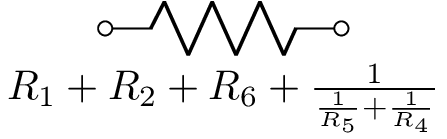
simplify(select, ignore, passes, series, parallel, dangling, explain, modify) Simplifies netlist by combing components in series and parallel and by removing dangling components. select is a list or set of the component names to consider; if None all the netlist components are considered for simplification. ignore is a list or set of components to ignore in the simplification. passes is the number of simplification iterations to perform. If zero, iterations continue until no more simpliciations are found. series enables series combination (default True). parallel enables parallel combination (default True). dangling enables dangling componet removal (default False). If explain is True, a description of each simplification is printed. If modify is False, the netlist is not modified.
simplify_series(select, ignore, passes) Simplifies netlist with components in series. See simplify for a description of the arguments.
simplify_parallel(select, ignore, passes) Simplifies netlist with components in parallel. See simplify for a description of the arguments.
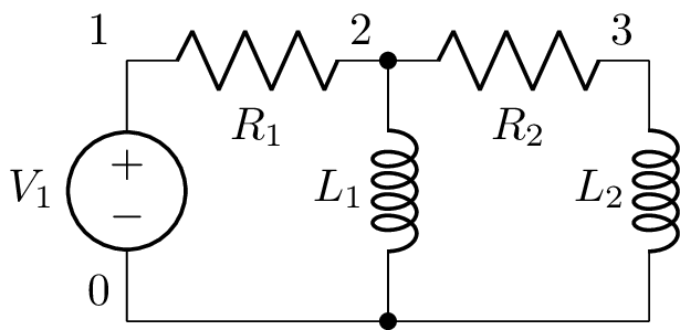
state_space(node_voltages, branch_currents) Generates a state-space representation (see State-space analysis) where node_voltages is a list of node names to use as voltage outputs (if None use all nodes) and branch_currents is a list of component names to use as branch current outputs (if None use all the components). Here’s an example:
>>> cct = Circuit('cct.sch')
>>> ss = cct.state_space(node_voltages=['1', '3'], branch_currents=['L1', 'L2'])
state_space_model() Creates a state-space model by replacing inductors with current sources and capacitors with voltage sources, see State-space analysis.
subs(subs_dict) Substitutes symbolic values in the netlist using a dictionary of symbols subs_dict. For example,
>>> cct = Circuit("""
... V1 1 0 Vs
... R1 1 2
... L1 2 0""")
>>> cct2 = cct.subs({'Vs': 10, 'L1': 3})
>>> cct2
V1 1 0 10
R1 1 2
L1 2 0 3
switching_times(tmax) Returns sorted list of times when switches become active if they are before tmax (default 1e12). For example,
>>> cct = Circuit("""
... SW1 1 2 no
... SW2 2 3 no 1
... SW3 3 4 nc 2""")
>>> cct.switching_times()
[0.0, 1.0, 2.0]
sympify(ignore) Converts numerical values to symbolic values except for component names specified by ignore. For example,
>>> cct = Circuit("""
... R 1 2 3
... C1 2 3 4
... C2 3 4 5 6
... L 4 5 7 8""")
>>> cct.sympify()
R 1 2
C1 2 3
C2 3 4 C2 v0_C2
L 4 5 L i0_L
>>> cct.sympify().subs(cct.defs())
R 1 2 3
C1 2 3 4
C2 3 4 5 6
L 4 5 7 8
Note how the initial values are named. See also defs() and subs().
unconnected_nodes Returns list of names of nodes that are unconnected
unreachable_nodes(node) Returns list of names of nodes that have no path to node.
Circuit two-port methods
Circuits have a number of two-port methods, primarily for determining transfer functions. The ports are specified by component name or a tuple of node names. Note, currents are defined to be flowing into the positive node of a port:
Here’s an example:
>>> a = Circuit("""
... P1 1 0
... R1 1 2
... R2 2 0
... R3 2 3
... P2 3 0""")
>>> a.voltage_gain(1, 0, 3, 0)
  R₂
───────
R₁ + R₂
>>> a.current_gain('P1', 'P2')
 -R₂
───────
R₂ + R₃
>>> a.transimpedance('P1', (3, 0))
R₂
>>> tpz = a.twoport('P1', 'P2', model='Z')
>>> tpz.voltage_gain
  R₂
───────
R₁ + R₂
Note, the currents are considered to be flowing into the positive nodes as is the convention with two-ports. Thus the input and output currents have opposite directions and so a piece of wire has a current gain of -1. Similarly the transadmittance of a resistor of resistance R is -1 / R.
The methods are:
transfer(N1p, N1m, N2p, N2m) Returns the s-domain transfer function V2(s) / V1(s), for the ports defined by nodes N1p, N1m, N2p, and N2m where V1 = V[N1p] - V[N1m] and V2 = V[N2p] - V[N2m]. This is an alias for voltage_gain(). The ports can also be specified using a component name or a tuple of node names, for example,
>>> H1 = cct.transfer('R1', 'L1')
>>> H2 = cct.transfer('R1', (2, 0))
voltage_gain(N1p, N1m, N2p, N2m) Returns the s-domain transfer function V2(s) / V1(s), for the ports defined by nodes N1p, N1m, N2p, and N2m where V1 = V[N1p] - V[N1m] and V2 = V[N2p] - V[N2m]. See also transfer() and Voltage gain.
current_gain(N1p, N1m, N2p, N2m) Returns the s-domain transfer function I2(s) / I1(s), for the ports defined by nodes N1p, N1m, N2p, and N2m. I1(s) is a test current injected into node N1p from node N1m. I2(s) is the short-circuit current flowing into N2p from N1p as is the convention with two-ports. See also transfer() and Current gain.
transadmittance(N1p, N1m, N2p, N2m) Returns the s-domain transadmittance function I2(s) / V1(s), for the ports defined by nodes N1p, N1m, N2p, and N2m. V1(s) is a test voltage applied between nodes N1p and N1m. I2(s) is the short-circuit current flowing into N2p from N1p as is the convention with two-ports. See also transfer() and Transadmittance.
transimpedance(N1p, N1m, N2p, N2m) Returns the s-domain transimpedance function V2(s) / I1(s), for the ports defined by nodes N1p, N1m, N2p, and N2m. I1(s) is a test current injected into node N1p from node N1m. V2(s) is the open-circuit voltage measured between N2p and N1p. See also transfer() and Transimpedance.
twoport(N1p, N1m, N2p, N2m, model=’B’) Returns an s-domain two-port model defined by nodes N1p, N1m, N2p, and N2m, where I1 is the current flowing into N1p and out of N1m, I2 is the current flowing into N2p and out of N2m, V1 = V[N1p] - V[N1m], and V2 = V[N2p] - V[N2m]. model can be A, B, G, H, Y, or Z.
Aparams(N1p, N1m, N2p, N2m) Returns the two-port A-parameters matrix for the two-port defined by nodes N1p, N1m, N2p, and N2m, where I1 is the current flowing into N1p and out of N1m, I2 is the current flowing into N2p and out of N2m, V1 = V[N1p] - V[N1m], and V2 = V[N2p] - V[N2m]. See A-parameters (ABCD) and twoport().
Bparams(N1p, N1m, N2p, N2m) Returns the two-port B-parameters matrix. See B-parameters (inverse ABCD) and twoport().
Gparams(N1p, N1m, N2p, N2m) Returns the two-port G-parameters matrix. See G-parameters (inverse hybrid) and twoport().
Hparams(N1p, N1m, N2p, N2m) Returns the two-port H-parameters matrix. See H-parameters (hybrid) and twoport().
Sparams(N1p, N1m, N2p, N2m) Returns the two-port S-parameters matrix. See S-parameters (scattering) and twoport().
Tparams(N1p, N1m, N2p, N2m) Returns the two-port T-parameters matrix. See T-parameters (scattering transfer) and twoport().
Yparams(N1p, N1m, N2p, N2m) Returns the two-port Y-parameters matrix. See Y-parameters (admittance) and twoport().
Zparams(N1p, N1m, N2p, N2m) Returns the two-port Z-parameters matrix. See Z-parameters (impedance) and twoport().
ladder(N1p, N1m, N2p, N2m) Returns an s-domain two-port model, for circuits with a ladder toplogy, defined by nodes N1p, N1m, N2p, and N2m, where V1 = V[N1p] - V[N1m], and V2 = V[N2p] - V[N2m]. Note, N1m has to be the same as N2m.
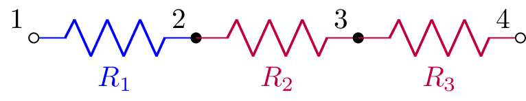
The ladder() method is useful for large circuits with an unbalanced ladder topology since it does not compute all the node voltages of the circuit and so is much faster than the other methods. For example, consider the ladder network:
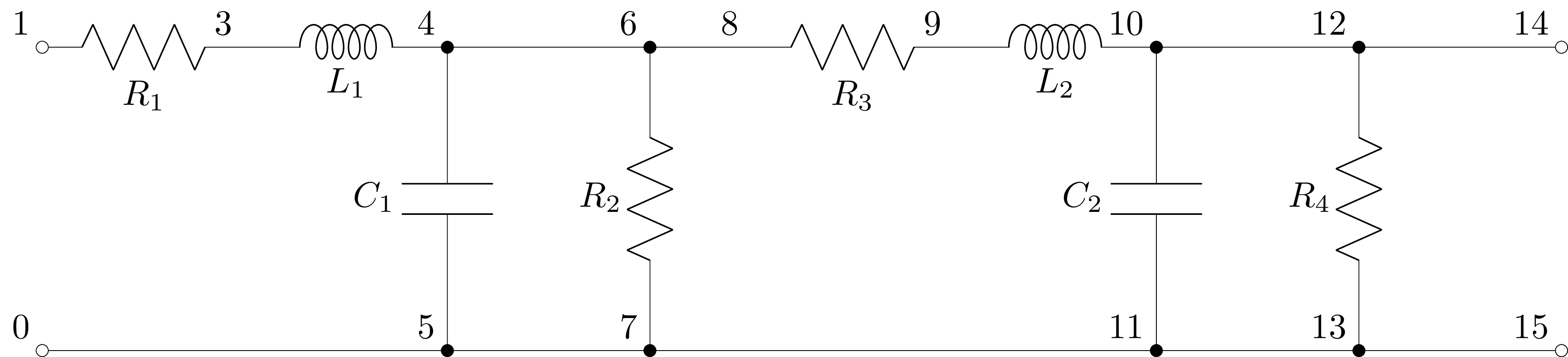
The voltage gain transfer function can be found using:
>>> ladder = cct.ladder(1, 0, 14, 0)
>>> ladder
Ladder(R(R1) + L(L1), C(C1) | R(R2), R(R3) + L(L2), C(C2) | R(R4))
>>> H = ladder.voltage_gain
Note, if the extracted ladder network is only a subsection of the original circuit, the voltage gain will not be correct due to the neglected loading of the ignored components. For example:
>>> subladder = cct.ladder(1, 0, 6, 0)
>>> subladder
Ladder(R(R1) + L(L1), C(C1) | R(R2))
>>> subladder.voltage_gain.simplify()
                R₂
──────────────────────────────
R₂ + (L₁⋅s + R₁)⋅(C₁⋅R₂⋅s + 1)
This has ignored the components R3, L2, C2, and R4.
Circuit multi-port methods
Yparamsn(N1p, N1m, N2p, N2m, …) Returns the n-port Y-parameters matrix. See Y-parameters (admittance).
Zparamsn(N1p, N1m, N2p, N2m, …) Returns the n-port Z-parameters matrix. See Z-parameters (impedance).
Circuit components
A Component object is obtained from a Circuit object using member notation. For example,
>>> cpt = cct.R1
Alternatively, a Component object can be obtained using array notation. For example,
>>> cpt = cct['R1']
Component attributes
Each Component object has a number of attributes, including:
V transform-domain voltage across component (use V(t) to get the time-domain voltage or V(s) to get the Laplace domain voltage)
I transform-domain current through component (use I(t) to get the time-domain current or I(s) to get the Laplace domain current)
v time-domain voltage across component
i time-domain current through component
Lcapy supports different Current sign convention s.
Note, the above attributes are influenced by other components in the circuit. The following attributes assume that the component is not in circuit:
Voc transform-domain open-circuit voltage; it is zero for passive components and infinite for current sources
Isc transform-domain short-circuit current (the current flowing through the component when it is short-circuited); it is zero for passive components and infinite for voltage sources
voc t-domain open-circuit voltage; it is zero for passive components and infinite for current sources
isc t-domain short-circuit current (the current flowing through the component when it is short-circuited); it is zero for passive components and infinite for voltage sources
B susceptance
G conductance
R resistance
X reactance
Y admittance
Z impedance
Ys s-domain generalized admittance
Zs s-domain generalized impedance
y t-domain impulse response of admittance
z t-domain impulse response of impedance
is_dc DC network
is_ac AC network
is_IVP initial value problem (at least one capacitor or inductor has an explicit initial condition)
is_causal causal response
v is the time-domain voltage difference across the component, for example:
>>> cct.R1.v
 -R₁⋅t
 ──────
   L₁
e      ⋅Heaviside(t)
i is the time-domain current through the component, for example:
>>> cct.R1.i
⎛      -R₁⋅t ⎞
⎜      ──────⎟
⎜        L₁  ⎟
⎜1    e      ⎟
⎜── - ───────⎟⋅Heaviside(t)
⎝R₁      R₁  ⎠
The V and I attributes provide the voltage and current as a superposition in the transform domains, for example,
>>> cct.V1.V
⎧   1⎫
⎨s: ─⎬
⎩   s⎭
The Y and Z attributes provide the generalized s-domain admittance and impedance of the component, for example,
>>> cct.L1.Z(s)
L₁⋅s
>>> cct.R1.Z(s)
R₁
The generalized s-domain driving point admittance and impedance can be found using dpY and dpZ, for example,
>>> cct.L1.dpZ(s)
 R₁⋅s
──────
    R₁
s + ──
    L₁
Note, this is the total impedance across L1, not just the impedance of the component as given by cct.L1.Z(s).
Here is the complete list of component attributes:
components dictionary of component lists
connected list of components connected to the component
has_ic initial conditions are specified
has_ac component is a source with an ac component
has_dc component is a source with a dc component
has_noisy component is a source with a noisy component
has_s_transient component is a source with a transient component defined in s-domain
has_t_transient component is a source with a transient component defined in time domain
has_transient component is a source with a transient component
is_ac component is a source that is only ac
is_causal source or component is causal
is_capacitor component is a capacitor
is_current_source component is a current source
is_dangling component has a node with fewer than 2 connections
is_dependent_source source is dependent
is_dc component is a source that is only dc
is_disconnected component has all nodes with fewer than 2 connections
is_inductor component is an inductor
is_independent_source source is independent
is_noisy component is a source that is only noisy
is_oneport component is a oneport
is_open_circuit component is an open-circuit
is_resistor component is a resistor
is_reactance component is a capacitor or inductor
is_source component is a source
is_twoport component is a twoport
is_voltage_source component is a voltage source
is_wire component is a wire
nodes list of nodes
node_names list of node names
nosim component is ignored for analysis
Component methods
norton() Creates Norton oneport object viewed from nodes of the component.
thevenin() Creates Thevenin oneport object viewed from nodes of the component.
oneport() Creates Thevenin or Norton oneport object as appropriate when viewed from nodes of the component.
transfer(cpt) Creates transfer function for the voltage across cpt divided by the voltage across the component.
connected() Returns list of components connected to this component (i.e., components that share a node).
is_connected(cpt) Returns True if connected to specified cpt (i.e., the components share a node).
in_parallel() Returns set of names of components in parallel with the component.
in_series() Returns set of names of components in series with the component.
noisy(T=’T’) Creates noisy model where resistors are replaced with a noiseless resistor and a noise voltage source.
noisy_except(resistors, T=’T’) Creates noisy model where all but the specified resistors are replaced with a noiseless resistance and a noise voltage source.
open_circuit() Applies open circuit in series with the component. The name of the open circuit component is returned.
short_circuit() Applies short circuit across the component using a 0 V voltage source. The name of the voltage source is returned.
Current sign convention
Lcapy supports three current sign conventions:
passive
Current flows into the positive node. This is the most common convention. However, note, the current of a source is negative:
>>> a = Circuit("""
... I1 1 0
... R1 1 0""")
>>> a.I1.i
-I₁
>>> a.R1.i
I₁
active
Current flows into the negative node. This is not common.
hybrid (default)
For a passive device (R, L, C), current flows into the positive node, and for a source (V, I), current flows out of the positive node.
The default current sign convention is passive. However, this is deprecated and will change to passive in a future release of Lcapy. The sign convention can be switched to passive using:
>>> from lcapy import rcparams
>>> rcparams['circuit.current_sign_convention] = 'passive'
Note, this will not change results previously computed and cached for a netlist.
Nodes
A Node object is obtained from a Circuit object using indexing notation. For example,
>>> n1 = cct[1]
>>> n2 = cct['2']
Node objects are also obtained from a Component object using the nodes attribute, for example,
>>> cct.R1.nodes
Node attributes
Nodes have many attributes including: name, v, V, dpY, and dpZ.
v is the time-domain voltage (with respect to the ground node 0).
V is a superposition of the node voltage in the different transform domains.
For example,
>>> cct[2].v
 -R₁⋅t
 ──────
   L₁
e      ⋅Heaviside(t)
dpY and dpZ return the driving-point admittance and impedance for the node with respect to ground, for example,
>>> cct[2].dpZ
 R₁⋅s
──────
    R₁
s + ──
    L₁
connected returns list of components connected to node
count returns number of components connected to node (excluding annotations and open-circuits)
is_dangling returns True if node count less than 2
is_ground returns True if node is a ground (starts with ‘0’)
Node methods
is_connected(node) Returns True if connected to specified node by a single component.
is_wired_to(node) Returns True if wired to specified node, directly or indirectly.
norton(node) Creates Norton oneport object with respect to specified node (default ground).
oneport(node) Creates oneport object with respect to specified node (default ground).
thevenin(node) Creates Thevenin oneport object with respect to specified node (default ground).
wired_to() Returns list of names of nodes that are wired to this node.
Oneports
A Oneport object is defined by a pair of nodes or by a component name. There are three circuit methods that will create a Oneport object from a Circuit object:
thevenin(Np, Nm) Creates a series combination of a voltage source and an impedance.
norton(Np, Nm) Creates a parallel combination of a current source and an impedance.
oneport(Np, Nm) Creates either a Norton model, Thevenin model, source, or impedance as appropriate.
A Oneport object is a Network object so shares the same attributes and methods, see Network attributes and Network methods.
Here’s an example of creating and using a Oneport object:
>>> cct = Circuit("""
>>> R1 3 2
>>> L 2 1
>>> C 1 0
>>> R2 3 0""")
>>> o = cct.oneport('R1')
Alternatively, a Oneport object can be created using a pair of nodes:
>>> o = cct.oneport(3, 2)
A third way is from a node object and another node name, for example,
>>> o = a[3].oneport(2)
Here’s an example,
>>> cct = Circuit("""
>>> R1 3 2
>>> L 2 1
>>> C 1 0
>>> R2 3 0""")
>>> cct.oneport('R1').Z(omega)
        ⎛   2   ⅉ⋅R₂⋅ω    1 ⎞
 C⋅L⋅R₁⋅⎜- ω  + ────── + ───⎟
        ⎝         L      C⋅L⎠
──────────────────────────────
       2
- C⋅L⋅ω  + ⅉ⋅C⋅ω⋅(R₁ + R₂) + 1
>>> cct.oneport('R1').Z(s)
        ⎛ 2   R₂⋅s    1 ⎞
 C⋅L⋅R₁⋅⎜s  + ──── + ───⎟
        ⎝      L     C⋅L⎠
──────────────────────────
     2
C⋅L⋅s  + C⋅s⋅(R₁ + R₂) + 1
Netlist evaluation
The circuit node voltages are determined using Modified Nodal Analysis (MNA). This is performed lazily as required with the results cached.
When a circuit has multiple independent sources, the circuit is decomposed into a number of sub-circuits; one for each source type. Again, this is performed lazily as required. Each sub-circuit is evaluated independently and the results are summed using the principle of superposition. For example, consider the circuit
>>> cct = Circuit("""
... V1 1 0 {1 + u(t)}
... R1 1 2
... L1 2 0""")
In this example, V1 can be considered the superposition of a DC source and a transient source. The approach Lcapy uses to solve the circuit can be found using the describe method:
>>> cct.describe()
This is solved using superposition.
DC analysis is used for source V1.
Laplace analysis is used for source V1.
For the curious, the sub-circuits can be found with the subcircuits attribute:
>>> cct.subcircuits
{'dc': V1 1 0 dc {1}
       R1 1 2
       L1 2 0 L_1,
's': V1 1 0 {Heaviside(t)}
     R1 1 2
     L1 2 0 L_1
}
Here the first sub-circuit is solved using DC analysis and the second sub-circuit is solved using Laplace analysis in the s-domain.
The properties of each sub-circuit can be found with the analysis attribute:
>>> cct.sub['dc'].analyse()
{'ac': False,
'causal': False,
'control_sources': [],
'dc': True,
'dependent_sources': [],
'has_s': False,
'has_ic': False,
'independent_sources': ['V1'],
'ivp': False,
'time_domain': False,
'zeroic': True}
Netlist decomposition and transformation
During circuit analysis, Lcapy decomposes netlists into dc, ac, transient, and noise sub-netlists. These are solved independently and then the total result is found from superposition.
Parts of the decomposition can be selected using the dc(), ac(), transient(), and noise() methods. These methods return a modified netlist where the independent source values are dc, ac, transient, and noise, respectively. The transient() method returns the transient components in the time-domain.
The method, laplace(), converts all the independent source values into the Laplace-domain and optionally adds initial conditions to capacitors and inductors. Similarly, time() converts all the independent source values into the time-domain.
For example, consider the netlist:
>>> cct = Circuit("""W 1 0; down
V1 1 2 dc; right
V2 2 3 ac; right
V3 3 4 {v(t)}; right
V4 4 5 noise; right
V5 5 6 {1 + u(t)}; right
R 6 0_6; down
W 0 0_6; right""")
The dc() method produces:
>>> cct.dc()
W 1 0; down
V1 1 2 dc; right
V2 2 3 dc 0; right
V3 3 4 dc 0; right
V4 4 5 dc 0; right
V5 5 6 dc 1; right
R 6 0_6; down
W 0 0_6; right
Here all the independent voltage sources only have the DC value of the original sources. The voltage sources with a zero value can be converted to wires using the kill_zero() method, for example:
>>> cct.dc().kill_zero()
W 1 0; down
V1 1 2 dc; right
W 2 3; right
W 3 4; right
W 4 5; right
V5 5 6 dc 1; right
R 6 0_6; down
W 0 0_6; right
Simplification
Netlists have simplification methods : remove_dangling(), remove_dangling_wires(), remove_disconnected(), simplify_series(), simplify_parallel(), and simplify(). The latter is a generic method; it repeatedly calls simplify_series() and simplify_parallel() until no changes can be made. The number of iterations is controlled by the passes argument.
Each of the netlist simplification methods have an explain argument, If this is True, the simplification steps are printed. There is also a modify argument. If this is False, the modifications are not performed.
Here’s an example netlist:
>>> a = Circuit("""
... R1 1 2; right
... R2 2 3; right
... W 3 3a; up=0.5
... W 3 3b; down=0.5
... R4 3a 4a; right
... R5 3b 4b; right
... W 4 4a; up=0.5
... W 4 4b; down=0.5
... R6 4 5; right
... ; draw_nodes=connections, label_nodes=none, label_ids=none""")
with a schematic:
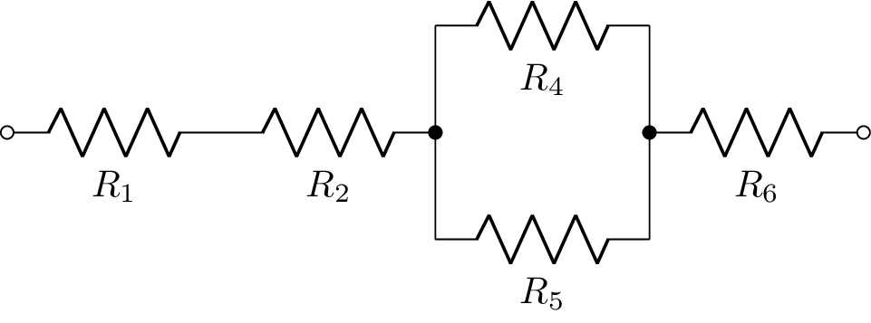
R1 and R2 can be combined in series using:
>>> b = a.simplify_series()
with a schematic:
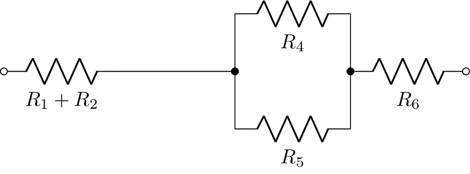
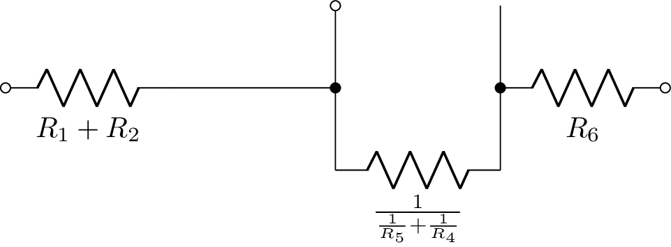
R3 and R4 can be combined in parallel using:
>>> c = b.simplify_parallel()
with a schematic:
These operations can be repeatedly executed until no further series or parallel combinations can be found. Alternatively, the simplify() method can be employed:
>>> d = a.simplify()
with a schematic:
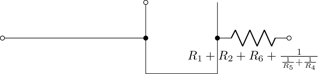
The dangling wires can be removed using the remove_dangling_wires() method:
>>> e = d.remove_dangling_wires()
with a schematic:
Netlist analysis examples
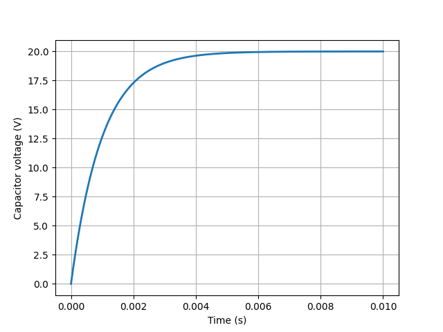
V-R-C circuit (1)
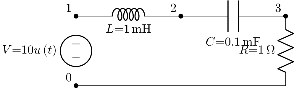
This example plots the transient voltage across a capacitor in a series R-L circuit:

from lcapy import Circuit

cct = Circuit("""
V 1 0 step 20
R 1 2 10
C 2 0 1e-4
""")

import numpy as np
t = np.linspace(0, 0.01, 1000)
vc = cct.C.v.evaluate(t)

from matplotlib.pyplot import subplots, savefig
fig, ax = subplots(1)
ax.plot(t, vc, linewidth=2)
ax.set_xlabel('Time (s)')
ax.set_ylabel('Capacitor voltage (V)')
ax.grid(True)

savefig('circuit-VRC1-vc.png')
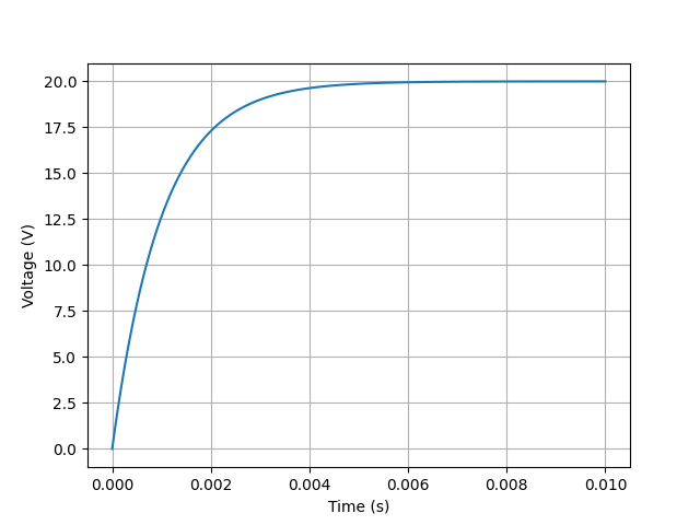
V-R-C circuit (2)
This example is the same as the previous example but it uses an alternative method of plotting.
from lcapy import Circuit

cct = Circuit("""
V 1 0 step 20
R 1 2 10
C 2 0 1e-4
""")

vc = cct.C.v

import numpy as np
t = np.linspace(0, 0.01, 1000)

from matplotlib.pyplot import subplots, savefig
fig, ax = subplots(1)
vc.plot(t, axes=ax)

savefig('circuit-VRC2-vc.png')
V-R-L-C circuit (1)
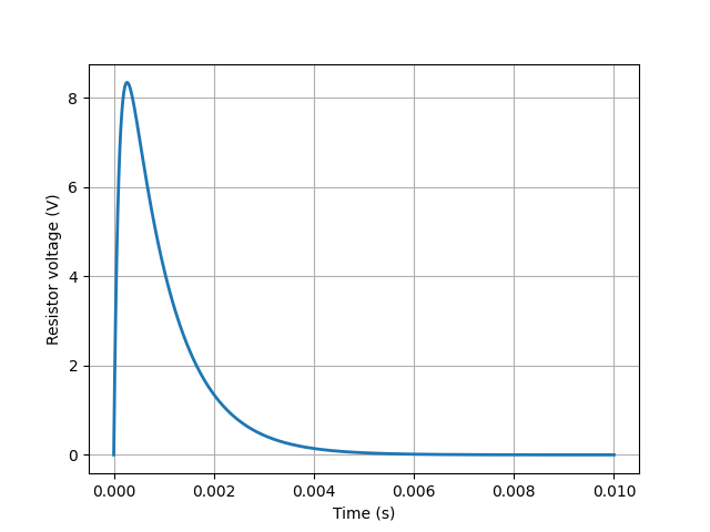
This example plots the transient voltage across a resistor in a series R-L-C circuit:
from lcapy import Circuit
cct = Circuit("""
V 1 0 step 10; down
L 1 2 1e-3; right, size=1.2
C 2 3 1e-4; right, size=1.2
R 3 0_1 10; down
W 0 0_1; right
""")

import numpy as np
t = np.linspace(0, 0.01, 1000)
vr = cct.R.v.evaluate(t)

from matplotlib.pyplot import subplots, savefig
fig, ax = subplots(1)
ax.plot(t, vr, linewidth=2)
ax.set_xlabel('Time (s)')
ax.set_ylabel('Resistor voltage (V)')
ax.grid(True)

savefig('circuit-VRLC1-vr.png')
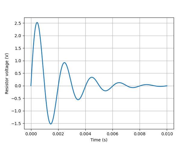
V-R-L-C circuit (2)
This is the same as the previous example but with a different resistor value giving an underdamped response:
from lcapy import Circuit
cct = Circuit("""
V 1 0 step 10; down
L 1 2 1e-3; right, size=1.2
C 2 3 1e-4; right, size=1.2
R 3 0_1 1; down
W 0 0_1; right
""")

import numpy as np
t = np.linspace(0, 0.01, 1000)
vr = cct.R.v.evaluate(t)

from matplotlib.pyplot import subplots, savefig
fig, ax = subplots(1)
ax.plot(t, vr, linewidth=2)
ax.set_xlabel('Time (s)')
ax.set_ylabel('Resistor voltage (V)')
ax.grid(True)

savefig('circuit-VRLC2-vr.png')
Mechanical netlists
LTI mechanical networks comprising masses, springs, and dampers can be simulated. Lcapy uses the mechanical-electrical analogue I (mobility or admittance analogue) where voltage is equivalent to speed and current is equivalent to force. Thus a mass is analogous to a capacitor, a spring is analogous to a inductor, and a damper (dashpot) is analogous to a resistor.
With this analogue d’Alemberts law is equivalent to Kirchhoff’s current law. Thus a point in the mechanical system is equivalent to a node in the electrical circuit. Note, that capacitors representing masses must have one terminal grounded.
- For example,
>>> a = Circuit("""
k 1 2; right
r 2 3; right
m 3 4; right""")
>>> Zm = a.admittance(1, 4)
>>> Zm
    k⋅s
────────────
k⋅s   k    2
─── + ─ + s
 r    m
The mechanical-electrical analogue II (impedance analogue) has the advantage that mechanical impedance is equivalent to electrical impedance. However, series mechanical components need to be modelled as parallel electrical components and vice-versa.
Transfer functions
Transfer functions are calculated for LTI systems in the Laplace domain with independent sources killed (voltage sources become short circuits and current sources become open circuits) and initial conditions set to zero. There are four types of transfer function: voltage gain, current gain, transimpedance, and transadmittance. In each case, the network is considered a two-port network, with an input port and an output port. Positive currents are assumed to flow into the positive node of a port.

Voltage gain
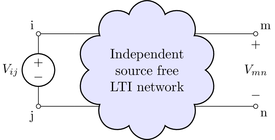
The voltage gain transfer function is defined as
\(H_{ijmn}(s) = \left.\frac{V_{mn}(s)}{V_{ij}(s)}\right|_{\mbox{zero ICs}}\)
where \(V_{ij}(s)\) is the Laplace domain voltage of a source applied between nodes \(i\) and \(j\) and \(V_{mn}(s)\) is the Laplace domain open-circuit voltage measured between nodes \(m\) and \(n\). This assumes that independent sources in the network are killed and that the initial conditions (capacitor voltages and inductor currents) are set to zero.
Current gain
The current gain transfer function is defined as
\(G_{ijmn}(s) = \left.\frac{I_{mn}(s)}{I_{ij}(s)}\right|_{\mbox{zero ICs}}\)
where \(I_{ij}(s)\) is the Laplace domain current of a source applied between nodes \(i\) and \(j\) and \(I_{mn}(s)\) is the Laplace domain short-circuit current measured between nodes \(m\) and \(n\). This assumes that independent sources in the network are killed and that the initial conditions (capacitor currents and inductor currents) are set to zero. Note, due to the definition of current flow, the current gain is -1 if the input port is the same as the output port.
Transimpedance
The transimpedance transfer function is defined as
\(Z_{ijmn}(s) = \left.\frac{V_{mn}(s)}{I_{ij}(s)}\right|_{\mbox{zero ICs}}\)
where \(I_{ij}(s)\) is the Laplace domain current of a source applied between nodes \(i\) and \(j\) and \(V_{mn}(s)\) is the Laplace domain open-circuit voltage measured between nodes \(m\) and \(n\). This assumes that independent sources in the network are killed and that the initial conditions (capacitor voltages and inductor currents) are set to zero.
Transadmittance

The transadmittance transfer function is defined as
\(Y_{ijmn}(s) = \left.\frac{I_{mn}(s)}{V_{ij}(s)}\right|_{\mbox{zero ICs}}\)
where \(V_{ij}(s)\) is the Laplace domain voltage of a source applied between nodes \(i\) and \(j\) and \(I_{mn}(s)\) is the Laplace domain short-circuit current measured between nodes \(m\) and \(n\). This assumes that independent sources in the network are killed and that the initial conditions (capacitor voltages and inductor currents) are set to zero.