Overview
This document provides an overview of Lcapy’s capabilities. It assumes you know something about circuit theory. If you know nothing about circuit theory, see Circuit analysis for novices. If you want some complete examples, see Tutorials.
Introduction
Lcapy is a Python package for symbolic linear circuit analysis and signal processing. It can also simulate circuits using numerical integration. Lcapy can only symbolically analyse linear, time invariant networks. In other words, networks comprised of basic circuit components (R, L, C, etc.) that do not vary with time. However, changes in circuit topology (e.g., switching circuits) can be analysed as a sequence of initial value problems.
Networks and circuits can be described using netlists or combinations of network elements. These can be drawn semi-automatically (see Schematics).
As well as performing circuit analysis, Lcapy can output the system of equations for mesh analysis, nodal analysis, modified nodal analysis, and state-space analysis (see Mesh analysis, Nodal analysis, Modified nodal analysis, and State-space analysis).
Lcapy cannot directly analyse non-linear devices such as diodes or transistors although it does support simple opamps without saturation. Nevertheless, it can draw them! Lcapy can generate text-book quality schematics using vector graphics (unlike the bit-mapped graphics used in this document).
Lcapy uses SymPy (symbolic Python) for its values and expressions and thus the circuit analysis can be performed symbolically. See http://docs.sympy.org/latest/tutorial/index.html for the SymPy tutorial.
Lcapy can perform many linear circuit analysis operations, including:
Solve linear circuits and networks symbolically (including time-variant circuits with switches)
Generate high-quality semi-automated schematics from netlists
Generate systems of equations for nodal, modified nodal, and mesh analysis
Perform state-space analysis
Perform Laplace, Fourier, Z, discrete-time Fourier, and discrete Fourier transforms
Track units of expressions for dimensional analysis
Analyse two-port networks (A, B, G, H, S, T, Y, and Z)
Perform Norton/Thevenin and wye/delta transforms
Analyse poly-phase systems
Perform time-stepping simulation for numerical circuit analysis (see Numerical simulation)
Generate many forms of plot (Bode, Nichols, Nyquist, pole-zero, etc.) with automatic axis labelling
Perform network synthesis given an immitance expression
Approximate continuous-time systems as discrete-time
Convert expressions into many forms (ZPK, partial fraction, etc.)
Parameterize an expression
Estimate numeric parameters of an expression (see Parameter estimation)
If you need to model a non-linear circuit numerically using Python, see PySpice (https://pypi.org/project/PySpice/).
Preliminaries
Before you can use Lcapy you need to install the Lcapy package (see Installation) or set PYTHONPATH to find the Lcapy source files.
Then fire up your favourite python interpreter, for example, ipython:
>>> ipython --pylab
Alternatively, you can use a Jupyter notebook (https://jupyter.org/).
Conventions
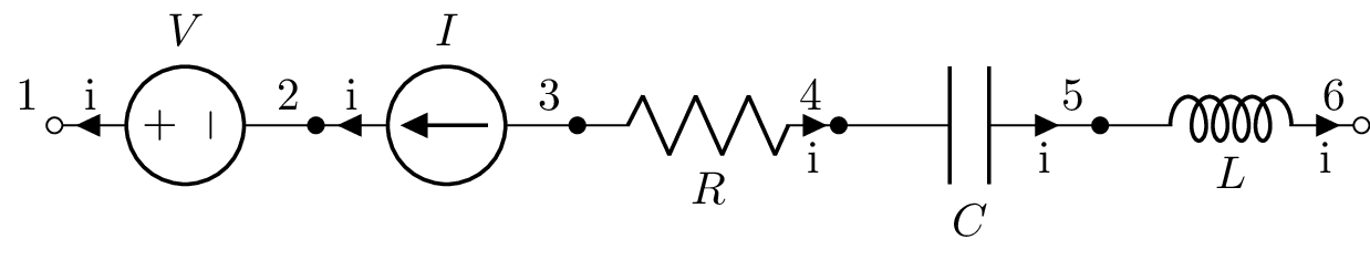
Lcapy uses the passive sign convention. Thus for a passive device (R, L, C), current flows into the positive node, and for a source (V, I), current flows out of the positive node.
Expressions
Lcapy defines a number of domain variables corresponding to different domains (see Domain variables):
t – time domain
f – Fourier (frequency) domain
F – normalised Fourier domain
s – Laplace (complex frequency) domain
omega – angular Fourier domain
Omega – normalised angular Fourier domain
jf – frequency response domain
jomega (or jw) – angular frequency response domain
n – discrete-time domain
k – discrete-frequency domain
z – z-domain
Expressions (see Expressions) can be formed using these symbols. For example, a time-domain expression can be created using:
>>> from lcapy import t, delta, u
>>> v = 2 * t * u(t) + 3 + delta(t)
2⋅t⋅u(t) + δ(t) + 3
and a s-domain expression can be created using:
>>> from lcapy import s, j, omega
>>> H = (s + 3) / (s - 4)
>>> H
s + 3
─────
s - 4
Numbers in expressions are represented as rationals to avoid numerical problems with floating-point numbers. For example:
>>> x = t * 0.1
t
──
10
The ratfloat() method can convert the rational numbers in an expression into floating-point numbers:
>>> x.ratfloat()
0.1⋅t
This is useful for printing but should be avoided for analysis. The companion function floatrat() converts floating-point numbers back to rationals but due to loss of precision, the result can be unwieldy (see Numbers). Alternatively, the evalf() method can be used with an argument specifying the number of digits
>>> pi.evalf(10)
 3.141592654
Lcapy expressions have an associated domain (e.g., time domain or Laplace domain), an associated quantity (such as voltage or impedance), and units. For more details see Domains, Quantities, and Units. Here is a time-domain current example:
>>> I = current(3 * t)
>>> I.domain
'time'
>>> I.quantity
'current'
>>> I.units
A
Here is a Laplace-domain voltage example:
>>> V = voltage(3 * s)
>>> V.domain
'laplace'
>>> V.quantity
'voltage'
>>> V.units
V
──
Hz
By default, the units are not printed (for more details see Units).
Lcapy expressions have a number of other attributes (see Expression attributes) including:
numerator, N – numerator of rational function
denominator, D – denominator of rational function
magnitude – magnitude
angle – angle
real – real part
imag – imaginary part
conjugate – complex conjugate
sympy – the underlying SymPy expression
val – the expression evaluated as a Lcapy floating-point value (if possible)
cval – the expression evaluated as a Python floating-point complex number (if possible)
fval – the expression evaluated as a Python floating-point number (if possible)
and many generic methods (see Expression methods) including:
approximate() – attempt approximation of the expression (see Approximation)
evaluate() – evaluate at specified vector and return floating-point vector (see Evaluation)
estimate() – estimate parameters of an expression given numerical data (see Parameter estimation)
simplify() – attempt simplification of the expression (see Simplification)
rationalize_denominator() – multiply numerator and denominator by complex conjugate of denominator
divide_top_and_bottom(expr) – divides numerator and denominator by expr.
multiply_top_and_bottom(expr) – multiplies numerator and denominator by expr.
Here’s an example that uses these attributes and methods:
>>> from lcapy import s, j, omega
>>> H = (s + 3) / (s - 4)
>>> A = H(j * omega)
>>> A
j⋅ω + 3
───────
j⋅ω - 4
>>> A.rationalize_denominator()
 2
ω  - 7⋅j⋅ω - 12
───────────────
     2
    ω  + 16
>>> A.real
 2
ω  - 12
───────
 2
ω  + 16
>>> A.imag
 -7⋅ω
───────
 2
ω  + 16
>>> A.N
j⋅ω + 3
>>> A.D
j⋅ω - 4
>>> A.phase
     ⎛       2     ⎞
atan2⎝-7⋅ω, ω  - 12⎠
>>> A.magnitude
   __________________
  ╱  4       2
╲╱  ω  + 25⋅ω  + 144
─────────────────────
        2
       ω  + 16
Each domain has specific methods, including:
as_fourier() – Convert to Fourier domain
as_laplace() – Convert to Laplace (s) domain
as_time() – Convert to time domain
as_phasor() – Convert to phasor domain
Lcapy defines a number of functions (see Mathematical functions) that can be used in expressions, including:
u() – Heaviside’s unit step
H() – Heaviside’s unit step
delta() – Dirac delta
cos() – cosine
sin() – sine
sqrt() – square root
exp() – exponential
log10() – logarithm base 10
log() – natural logarithm
Expression formatting
Lcapy can format expressions in many ways (see Formatting methods). For example, it can represent expressions in partial fraction form:
>>> from lcapy import *
>>> G = 1 / (s**2 + 5 * s + 6)
>>> G.partfrac()
   1       1
- ───── + ─────
  s + 3   s + 2
Here’s an example of partial fraction expansion for a not strictly proper rational function:
>>> from lcapy import *
>>> H = 5 * (s + 5) * (s - 4) / (s**2 + 5 * s + 6)
>>> H.partfrac()
      70      90
5 + ───── - ─────
    s + 3   s + 2
The rational function can also be printed in ZPK (zero-pole-gain) form:
>>> H.ZPK()
5⋅(s - 4)⋅(s + 5)
─────────────────
 (s + 2)⋅(s + 3)
Here it is obvious that the poles are -2 and -3. These can also be found using the poles function:
>>> H.poles()
{-3: 1, -2: 1}
Here the number after the colon indicates how many times the pole is repeated.
Similarly, the zeros can be found using the zeros function:
>>> H.zeros()
{-5: 1, 4: 1}
Lcapy can also handle rational functions with a delay.
Inverse Laplace transforms
Lcapy can perform inverse Laplace transforms. Here’s an example for a strictly proper rational function:
>>> from lcapy import s
>>> H = 5 * (s - 4) / (s**2 + 5 * s + 6)
>>> H.partfrac()
  35      30
───── - ─────
s + 3   s + 2

>>> H.ILT()
      -2⋅t       -3⋅t
- 30⋅e     + 35⋅e      for t ≥ 0
or alternatively
>>> H(t)
      -2⋅t       -3⋅t
- 30⋅e     + 35⋅e      for t ≥ 0
Note that the unilateral inverse Laplace transform can only determine the result for \(t \ge 0\). If you know that the system is causal, then use:
>>> H(t, causal=True)
⎛      -2⋅t       -3⋅t⎞
⎝- 30⋅e     + 35⋅e    ⎠⋅Heaviside(t)
The Heaviside function is also known as the unit step. Alternatively, you can force the result to be causal:
>>> H(t).force_causal()
⎛      -2⋅t       -3⋅t⎞
⎝- 30⋅e     + 35⋅e    ⎠⋅Heaviside(t)
or remove the condition that \(t \ge 0\),
>>> H(t).remove_condition()
      -2⋅t       -3⋅t
- 30⋅e     + 35⋅e
When the rational function is not strictly proper, the inverse Laplace transform has Dirac deltas (and derivatives of Dirac deltas):
>>> from lcapy import s
>>> H = 5 * (s - 4) / (s**2 + 5 * s + 6)
>>> H.partfrac()
     70      90
5 + ───── - ─────
    s + 3   s + 2
>>> H.ILT(causal=True)
⎛      -2⋅t       -3⋅t⎞
⎝- 90⋅e     + 70⋅e    ⎠⋅Heaviside(t) + 5⋅DiracDelta(t)
Here’s another example of a strictly proper rational function with a repeated pole:
>>> from lcapy import s
>>> H = 5 * (s + 5) / ((s + 3) * (s + 3))
>>> H.ZPK()
5⋅(s + 5)
─────────
        2
 (s + 3)
>>> H.partfrac()
  5        10
───── + ────────
s + 3          2
        (s + 3)
>>> H.ILT(causal=True)
⎛      -3⋅t      -3⋅t⎞
⎝10⋅t⋅e     + 5⋅e    ⎠⋅Heaviside(t)
Rational functions with delays can also be handled:
>>> from lcapy import s, symbol, exp
>>> T = symbol('T')
>>> H = 5 * (s + 5) * (s - 4) / (s**2 + 5 * s + 6) * exp(-s * T)
>>> H.partfrac()
⎛      70      90 ⎞  -T⋅s
⎜5 + ───── - ─────⎟⋅e
⎝    s + 3   s + 2⎠
>>> H.ILT(causal=True)
⎛      2⋅T - 2⋅t       3⋅T - 3⋅t⎞
⎝- 90⋅e          + 70⋅e         ⎠⋅Heaviside(-T + t) + 5⋅DiracDelta(-T + t)
Lcapy can convert s-domain products to time domain convolutions, for example:
>>> from lcapy import expr
>>> expr('V(s) * Y(s)')(t, causal=True)
t
⌠
⎮ v(t - τ)⋅y(τ) dτ
⌡
0
Here the function expr converts a string argument to an Lcapy expression.
Lcapy can also recognise integrations and differentiations of arbitrary functions, for example:
>>> from lcapy import s, t
>>> (s * 'V(s)')(t, causal=True)
d
──(v(t))
dt

>>> ('V(s)' / s)(t, causal=True)
t
⌠
⎮ v(τ) dτ
⌡
0
These- expressions can also be written as:
>>> from lcapy import expr, t
>>> expr('s * V(s)')(t, causal=True)
>>> expr('V(s) / s')(t, causal=True)
or more explicitly:
>>> from lcapy import expr
>>> expr('s * V(s)').ILT(causal=True)
>>> expr('V(s) / s').ILT(causal=True)
Laplace transforms
Lcapy can perform Laplace transforms. Here’s an example:
>>> from lcapy import s, t
>>> v = 10 * t ** 2 + 3 * t
>>> v.LT()
3⋅s + 20
────────
    3
   s
There is a short-hand notation for the Laplace transform:
>>> v(s)
3⋅s + 20
────────
    3
   s
Note, Lcapy uses the \(\mathcal{L}_{-}\) unilateral Laplace transform whereas SymPy which uses the \(\mathcal{L}\) unilateral Laplace transform, see Laplace transforms. The key difference is for Dirac deltas (and their derivatives). Lcapy gives:
>>> delta(t)(s)
1
However, SymPy gives 0.5.
Phasors
Phasors are created with the phasor() function:
>>> s = phasor(-2 * j)
>>> s.time()
2⋅sin(ω⋅t)
The default angular frequency is omega but this can be specified:
>>> p = phasor(-j, omega=1)
>>> p(t)
sin(t)
Phasors can also be inferred from an AC signal:
>>> q = phasor(2 * sin(3 * t))
>>> q
-2⋅ⅉ
>>> q.omega
3
For more information on phasors see Phasors.
Frequency response
For steady-state signals, the s-domain can be converted to the angular frequency response domain:
>>> from lcapy import s, j, omega
>>> H = (s + 3) / (s - 4)
>>> A = H(jw)
>>> A
j⋅ω + 3
───────
j⋅ω - 4
The symbol jomega can be used instead of jw.
The angular frequency response domain is almost equivalent to the angular Fourier domain, see Frequency response and Fourier domains (jomega or omega).
Networks
Networks can be constructed using series and parallel combination of one-port network elements and other networks, see Networks.
Network elements
The basic circuit components are two-terminal (one-port) devices are:
I – current source
V – voltage source
R – resistor
G – conductor
C – capacitor
L – inductor
These are augmented by generic s-domain components:
Y – generic admittance
Z – generic impedance
Here are some examples of their creation:
>>> from lcapy import *
>>> R1 = R(10)
>>> C1 = C(10e-6)
>>> L1 = L('L_1')
Network element combination
Here’s an example of resistors in series:
>>> from lcapy import *
>>> R1 = R(10)
>>> R2 = R(5)
>>> Rtot = R1 + R2
>>> Rtot
R(10) + R(5)
>>> Rtot.simplify()
R(15)
Here R(10) creates a 10 ohm resistor and this is assigned to the variable R1. Similarly, R(5) creates a 5 ohm resistor and this is assigned to the variable R2. Rtot is the name of the network formed by connecting R1 and R2 in series. Calling the simplify method will simplify the network and combine the resistors into a single resistor equivalent.
Here’s an example of a parallel combination of resistors. Note that the parallel operator is | instead of the usual ||.
>>> from lcapy import *
>>> Rtot = R(10) | R(5)
>>> Rtot
R(10) | R(5)
>>> Rtot.simplify()
R(10/3)
The result can be performed symbolically, for example:
>>> from lcapy import *
>>> Rtot = R('R_1') | R('R_2')
>>> Rtot
R(R_1) | R(R_2)
>>> Rtot.simplify()
R(R_1*R_2/(R_1 + R_2))
>>> Rtot.simplify()
R(R₁) | R(R₂)
Here’s another example using inductors in series:
>>> from lcapy import *
>>> L1 = L(10)
>>> L2 = L(5)
>>> Ltot = L1 + L2
>>> Ltot
L(10) + L(5)
>>> Ltot.simplify()
L(15)
Finally, here’s an example of a parallel combination of capacitors:
>>> from lcapy import *
>>> Ctot = C(10) | C(5)
>>> Ctot
C(10) | C(5)
>>> Ctot.simplify()
C(15)
Impedances
Impedance is a frequency domain generalization of resistance, see Immittances.
Let’s consider a series R-L-C network:
>>> from lcapy import *
>>> n = R(4) + L(10) + C(20)
>>> n
R(4) + L(10) + C(20)
The phasor impedance can be determined as a function of angular frequency using:
>>> n.Z(jomega)
              ⅉ
10⋅ⅉ⋅ω + 4 - ────
             20⋅ω
Similarly, the generalized (s-domain) impedance can be determined using:
>>> n.Z(s)
    2         1
10⋅s  + 4⋅s + ──
              20
────────────────
       s
Impedance expressions are rational functions (of \(\omega\) or \(s\)) and can be formatted in a number of different ways, for example:
>>> n.Z(s).ZPK()
   ⎛      ____    ⎞ ⎛      ____    ⎞
   ⎜    ╲╱ 14    1⎟ ⎜    ╲╱ 14    1⎟
10⋅⎜s - ────── + ─⎟⋅⎜s + ────── + ─⎟
   ⎝      20     5⎠ ⎝      20     5⎠
────────────────────────────────────
                 s

>>> n.Z(s).standard()
            1
10⋅s + 4 + ────
           20⋅s
Here ZPK() prints the impedance in ZPK (zero-pole-gain) form while standard() prints the rational function as the sum of a polynomial and a strictly proper rational function.
The corresponding parallel R-L-C network yields:
>>> from lcapy import *
>>> n = R(5) | L(20) | C(10)
>>> n
R(5) | L(20) | C(10)
>>> n.Z(s)
        s
──────────────────
   ⎛ 2   s     1 ⎞
10⋅⎜s  + ── + ───⎟
   ⎝     50   200⎠

>>> n.Z(s).ZPK()
                s
──────────────────────────────────
   ⎛     1    7⋅j⎞ ⎛     1    7⋅j⎞
10⋅⎜s + ─── - ───⎟⋅⎜s + ─── + ───⎟
   ⎝    100   100⎠ ⎝    100   100⎠
>>> n.Z(s).canonical()
        s
──────────────────
   ⎛ 2   s     1 ⎞
10⋅⎜s  + ── + ───⎟
   ⎝     50   200⎠
>>> n.Y(s)
     2
200⋅s  + 4⋅s + 1
────────────────
      20⋅s
Notice how n.Y(s) returns the s-domain admittance of the network, the reciprocal of the impedance n.Z(s).
The frequency response can be evaluated numerically by specifying a vector of frequency values. For example:
>>> from lcapy import *
>>> from numpy import linspace
>>> n = Vstep(20) + R(5) + C(10)
>>> vf = linspace(0, 4, 400)
>>> Isc = n.Isc(f).evaluate(vf)
Then the frequency response can be plotted. For example:
>>> from matplotlib.pyplot import figure, show
>>> fig = figure()
>>> ax = fig.add_subplot(111)
>>> ax.loglog(f, abs(Isc), linewidth=2)
>>> ax.set_xlabel('Frequency (Hz)')
>>> ax.set_ylabel('Current (A/Hz)')
>>> ax.grid(True)
>>> show()
A simpler approach is to use the plot() method:
>>> from lcapy import *
>>> from numpy import linspace
>>> n = Vstep(20) + R(5) + C(10)
>>> vf = linspace(0, 4, 400)
>>> n.Isc(f).plot(vf, log_scale=True)
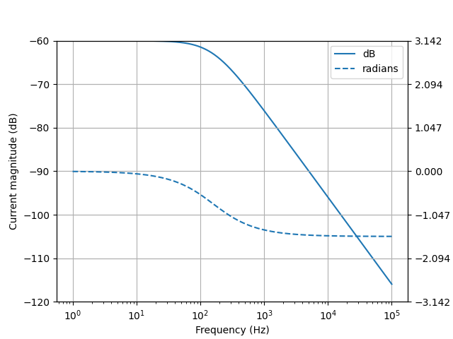
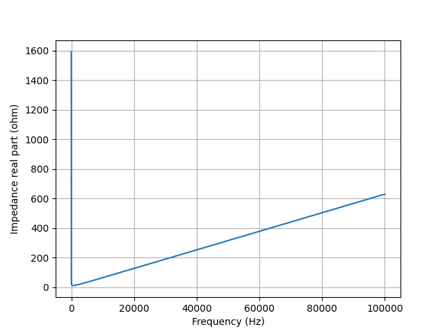
Here’s a complete example Python script to plot the impedance of a series R-L-C network:
from lcapy import *
from numpy import logspace
from matplotlib.pyplot import savefig

N = R(10) + C(1e-4) + L(1e-3)

vf = logspace(0, 5, 400)
N.Z(j2pif).magnitude.plot(vf)

savefig('series-RLC3-Z.png')
Simple transient analysis
Let’s consider a series R-C network in series with a DC voltage source
>>> from lcapy import *
>>> n = Vstep(20) + R(5) + C(10, 0)
>>> n
Vstep(20) + R(5) + C(10, 0)
>>> Voc = n.Voc(s)
>>> Voc
20
──
s
>>> n.Isc(s)
   4
────────
s + 1/50
>>> isc = n.Isc(t)
   -t
   ───
    50
4⋅ℯ   ⋅u(t)
Here n is network formed by the components in series, and n.Voc(s) is the open-circuit s-domain voltage across the network. Note, this is the same as the s-domain value of the voltage source. n.Isc(s) is the short-circuit s-domain voltage through the network and n.Isc(t) is the the time-domain response.
Of course, the previous example can be performed symbolically,
>>> from lcapy import *
>>> n = Vstep('V_1') + R('R_1') + C('C_1')
>>> n
Vstep(V₁) + R(R₁) + C(C)
>>> Voc = n.Voc(s)
>>> Voc
V₁
──
s
>>> n.Isc(s)
      V₁
──────────────
   ⎛      1  ⎞
R₁⋅⎜s + ─────⎟
   ⎝    C₁⋅R₁⎠
>>> isc = n.Isc(t)
>>> isc
     -t
    ─────
    C₁⋅R₁
V₁⋅ℯ     ⋅u(t)
──────────────
      R₁
The transient response can be evaluated numerically by specifying a vector of time values to the evaluate() method:
>>> from lcapy import *
>>> from numpy import linspace
>>> n = Vstep(20) + R(5) + C(10, 0)
>>> tv = linspace(0, 100, 400)
>>> isc = n.Isc(t).evaluate(tv)
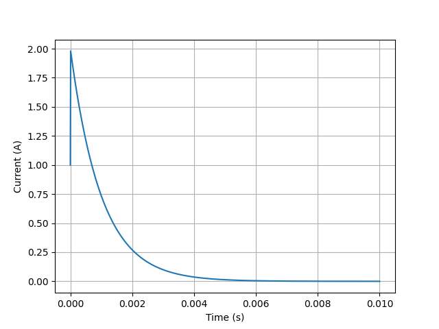
Then the transient response can be plotted. Alternatively, the plot() method can be used.
from lcapy import *
from numpy import linspace
from matplotlib.pyplot import savefig

N = Vstep(20) + R(10) + C(1e-4, 0)

vt = linspace(0, 0.01, 1000)
N.Isc(t).plot(vt)

savefig('series-VRC1-isc.png')
This produces:
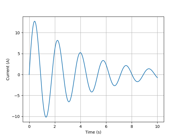
Here’s a complete example Python script of the short-circuit current through an underdamped series RLC network:
from lcapy import Vstep, R, L, C, t
from matplotlib.pyplot import savefig
from numpy import linspace

a = Vstep(10) + R(0.1) + C(0.4) + L(0.2, 0)

vt = linspace(0, 10, 1000)
a.Isc(t).plot(vt)

savefig('series-VRLC1-isc.png')
Transformations
A one-port network can be represented as a Thevenin network (a series combination of a voltage source and an impedance) or as a Norton network (a parallel combination of a current source and an admittance).
Here’s an example of a Thevenin to Norton transformation:
>>> from lcapy import *
>>> T = Vdc(10) + R(5)
>>> n = T.norton()
>>> n
G(1/5) | Idc(2)
Similarly, here’s an example of a Norton to Thevenin transformation:
>>> from lcapy import *
>>> n = Idc(10) | R(5)
>>> T = n.thevenin()
>>> T
R(5) + Vdc(50)
Two-port networks
The basic circuit components are one-port networks. They can be combined to create a two-port network. The simplest two-port is a shunt:
-----+----
     |
   +-+-+
   |   |
   |OP |
   |   |
   +-+-+
     |
-----+----
A more interesting two-port network is an L section (voltage divider):
  +---------+
--+   OP1   +---+----
  +---------+   |
              +-+-+
              |   |
              |OP2|
              |   |
              +-+-+
                |
----------------+----
This is comprised from any two one-port networks. For example:
>>> from lcapy import *
>>> R1 = R('R_1')
>>> R2 = R('R_2')
>>> n = LSection(R1, R2)
>>> n.Vtransfer
R_2/(R_1 + R_2)
Here n.Vtransfer determines the forward voltage transfer function V_2(s) / V_1(s).
The open-circuit input impedance can be found using:
>>> n.Z1oc
R₁ + R₂
The open-circuit output impedance can be found using:
>>> n.Z2oc
R₂
The short-circuit input admittance can be found using:
>>> n.Y1sc
1
──
R₁
The short-circuit output admittance can be found using:
>>> n.Y2sc
R₁ + R₂
───────
 R₁⋅R₂
Two-port combinations
Two-port networks can be combined in series, parallel, series at the input with parallel at the output (hybrid), parallel at the input with series at the output (inverse hybrid), but the most common is the chain or cascade. This connects the output of the first two-port to the input of the second two-port.
For example, an L section can be created by chaining a shunt to a series one-port:
>>> from lcapy import *
>>> n = Series(R('R_1')).chain(Shunt(R('R_2')))
>>> n.Vtransfer
R_2/(R_1 + R_2)
Two-port matrices
Two-port networks can be parameterised by eight different two by two matrices, A, B, G, H, S, T, Y, Z. Each has their own merits (see http://en.wikipedia.org/wiki/Two-port_network).
Consider an L section comprised of two resistors:
>>> from lcapy import *
>>> n = LSection(R('R_1'), R('R_2'))
The different matrix representations can be shown using:
>>> n.Aparams
⎡R₁ + R₂    ⎤
⎢───────  R₁⎥
⎢   R₂      ⎥
⎢           ⎥
⎢  1        ⎥
⎢  ──     1 ⎥
⎣  R₂       ⎦
>>> n.Bparams
⎡ 1    -R₁  ⎤
⎢           ⎥
⎢-1   R₁    ⎥
⎢───  ── + 1⎥
⎣ R₂  R₂    ⎦
>>> n.Gparams
⎡   1       -R₂  ⎤
⎢───────  ───────⎥
⎢R₁ + R₂  R₁ + R₂⎥
⎢                ⎥
⎢   R₂     R₁⋅R₂ ⎥
⎢───────  ───────⎥
⎣R₁ + R₂  R₁ + R₂⎦
>>> n.Hparams
⎡R₁  1 ⎤
⎢      ⎥
⎢    1 ⎥
⎢-1  ──⎥
⎣    R₂⎦
>>> n.Yparams
⎡1      -1   ⎤
⎢──     ───  ⎥
⎢R₁      R₁  ⎥
⎢            ⎥
⎢-1   R₁ + R₂⎥
⎢───  ───────⎥
⎣ R₁   R₁⋅R₂ ⎦
>>> n.Zparams
⎡R₁ + R₂  R₂⎤
⎢           ⎥
⎣  R₂     R₂⎦
Note, some of the two-port matrices cannot represent a network. For example, a series impedance has a non specified Z matrix and a shunt impedance has a non specified Y matrix.
Netlists
Creating complicated networks by combining network elements soon becomes tedious. A simpler way is to describe the network (or circuit) using a netlist, see Netlists. Here’s an example of a resistor in series with a capacitor:
>>> cct = Circuit("""
... R 1 2
... C 2 0""")
Here the numbers represent node names although these can be alphanumeric as well.
Transfer functions
Transfer functions can be created from netlists using the transfer() method. Here’s an example for an RC low-pass filter:
>>> cct = Circuit("""
... R 1 2
... C 2 0""")
>>> H = cct.transfer(1, 0, 2, 0)
>>> H
 ⎛ 1 ⎞
 ⎜───⎟
 ⎝C⋅R⎠
───────
     1
s + ───
    C⋅R
Transfer functions are defined in the Laplace domain but can be converted to the a angular frequency response domain:
>>> H(jw)
         1
───────────────
    ⎛       1 ⎞
C⋅R⋅⎜ⅉ⋅ω + ───⎟
    ⎝      C⋅R⎠
The transfer() method determines the ratio of the output to the input Laplace voltage, where the voltages are calculated from the given the input and output nodes. An alternative syntax is to specify the components that the voltages are measured over, for example:
>>> H = cct.transfer('R', 'C')
Furthermore, a component and a tuple of nodes can be used instead:
>>> H = cct.transfer('R', (2, 0))
Transfer functions can also be created in a similar manner to Matlab, either using lists of numerator and denominator coefficients:
>>> from lcapy import *
>>> H1 = tf(0.001, [1, 0.05, 0])
>>> H1
    0.001
───────────────
     2
1.0⋅s  + 0.05⋅s
from lists of poles and zeros (and optional gain):
>>> from lcapy import *
>>> H2 = zp2tf([], [0, -0.05])
>>> H2
     0.001
───────────────
     2
1.0⋅s  + 0.05⋅s
or symbolically:
>>> from lcapy import *
>>> H3 = 0.001 / (s**2 + 0.05 * s)
>>> H3
     0.001
───────────────
     2
1.0⋅s  + 0.05⋅s
In each case, parameters can be expressed numerically or symbolically, for example:
>>> from lcapy import *
>>> H4 = zp2tf(['z_1'], ['p_1', 'p_2'])
>>> H4
       s - z₁
───────────────────
(-p₁ + s)⋅(-p₂ + s)
Finally, transfer functions can also be found from the ratio of two s-domain quantities such as voltage or current with zero initial conditions. Here’s an example using an arbitrary input voltage V(s):
>>> from lcapy import Circuit
>>> cct = Circuit("""
... V1 1 0 {V(s)}
... R1 1 2
... C1 2 0 C1 0""")
>>> cct[2].V(s)
    V(s)
───────────
C₁⋅R₁⋅s + 1

>>> H = cct[2].V(s) / cct[1].V(s)
>>> H
     1
───────────
C₁⋅R₁⋅s + 1
The corresponding impulse response can found from an inverse Laplace transform:
>>> H.ILT(causal=True)
  -t
 ─────
 C₁⋅R₁
e     ⋅Heaviside(t)
───────────────────
       C₁⋅R₁
or more simply using:
>>> H(t, causal=True)
  -t
 ─────
 C₁⋅R₁
e     ⋅Heaviside(t)
───────────────────
       C₁⋅R₁
Circuit analysis
The nodal voltages for a linear circuit can be found using Modified Nodal Analysis (MNA). This requires the circuit topology be entered as a netlist (see Netlists). This describes each component, its name, value, and the nodes it is connected to. This netlist can be read from a file or created dynamically, for example:
>>> from lcapy import Circuit
>>> cct = Circuit()
>>> cct.add('V1 1 0 step 10')
>>> cct.add('Ra 1 2 3e3')
>>> cct.add('Rb 2 0 1e3')
This creates a circuit comprised of a 10 V step voltage source connected to two resistors in series. The node named 0 denotes the ground which the other voltages are referenced to. Here’s a more compact way to specify the netlist:
>>> from lcapy import Circuit
>>> cct = Circuit("""
... V1 1 0 step 10
... Ra 1 2 3e3
... Rb 2 0 1e3""")
The circuit has an attribute for each circuit element (and for each node starting with an alphabetical character). These can be interrogated to find the voltage drop across an element or the current through an element, for example:
>>> cct.V1.V
10⋅u(t)
>>> cct.Rb.V
5⋅u(t)
──────
  2
The returned result is a superposition of expressions in the different transform domains. In this example, there is only a single time-domain component. If there are multiple components, they are displayed as a dictionary, keyed by the transform domains.
The superposition can be converted into a Laplace domain expression using:
>>> cct.V1.V(s)
 10
 ──
 s
or into a time domain expression using:
>>> cct.V1.V(t)
10
The current through a component is obtained with the I attribute. For a source the current is assumed to flow out of the positive node, however, for a passive device (R, L, C) it is assumed to flow into the positive node.
The voltage between a node and ground can be determined with the node name as an index, for example:
>>> cct[1].V(t)
10
>>> cct[2].V(t)
5
─
2
Since Lcapy uses SymPy, circuit analysis can be performed symbolically. This can be achieved by using symbolic arguments or by not specifying a component value. In the latter case, Lcapy will use the component name for its value. For example:
>>> cct = Circuit("""
... V1 1 0 step Vs
... R1 1 2
... C1 2 0""")
>>> cct[2].V(s)
        V_s
 ──────────────────
       ⎛ 2     s  ⎞
 C₁⋅R₁⋅⎜s  + ─────⎟
       ⎝     C₁⋅R₁⎠

>>> : cct[2].V(t)
⎛            -t  ⎞
⎜           ─────⎟
⎜           C₁⋅R₁⎟
⎝V_s - V_s⋅e     ⎠⋅Heaviside(t)
Transform domains
Lcapy analyses a linear circuit using a number of transform domains and the principle of superposition. Voltage and current signals are decomposed into a DC component, one or more AC components (one for each angular frequency), a transient component, and noise components (one for each noise source).
For example, consider:
>>> Voc = (Vdc(10) + Vac(20) + Vstep(30) + Vnoise(40)).Voc
>>> Voc
⎧                   30        ⎫
⎨dc: 10, n1: 40, s: ──, ω₀: 20⎬
⎩                   s         ⎭
Here the open-circuit voltage is decomposed into four parts (stored in a dictionary). The DC component is keyed by ‘dc’, the transient component is keyed by ‘s’ (since this is analysed in the Laplace or s-domain), the noise components are keyed by noise identifiers of the form ‘nx’ (where x is an integer), and the AC components are keyed by the angular frequency (the default is omega0). The different parts of a decomposition can also be accessed using attributes, for example:
>>> Voc.s
30
──
s
Note, this only returns the Laplace transform of the transient component of the decomposition. The full Laplace transform of the open-circuit voltage (ignoring the noise component) can be obtained using:
>>> from lcapy import s
>>> Voc(s)
   ⎛    2      2⎞
20⋅⎝2⋅ω₀  + 3⋅s ⎠
─────────────────
     ⎛  2    2⎞
   s⋅⎝ω₀  + s ⎠
Similarly, the time-domain representation (ignoring the noise component) can be determined using:
>>> from lcapy import t
>>> Voc(t)
20⋅cos(ω₀⋅t) + 30⋅u(t) + 10
Initial value problems
The initial voltage difference across a capacitor or the initial current through an inductor can be specified as an additional argument. For example:
>>> cct = Circuit("""
... V1 1 0 step Vs
... C1 2 1 C1 v0
... L1 2 0 L1 i0""")
>>> cct[2].V(s)
           ⎛        i₀          ⎞
(V_s + v₀)⋅⎜- ────────────── + s⎟
           ⎝  C₁⋅V_s + C₁⋅v₀    ⎠
─────────────────────────────────
             2     1
            s  + ─────
                 C₁⋅L₁
Note, the component values need to be specified as well as the initial value; thus C1 2 1 C1 v0 and not C1 2 1 v0 since the latter specifies the capacitance to be v0.
When an initial condition is detected, the circuit is analysed in the s-domain as an initial value problem. The values of sources are ignored for \(t<0\) and the result is only defined for \(t\ge 0\).
Mesh analysis
Lcapy can generate a system of equations using mesh analysis, see Mesh analysis.
Nodal analysis
Lcapy can generate a system of equations using nodal analysis, see Nodal analysis.
Modified nodal analysis
Lcapy uses modified nodal analysis for its calculations. For reactive circuits it does this independently for the DC, AC, and transient components and uses superposition to combine the results. For resistive circuits, it can perform this in the time-domain. For more details see Modified nodal analysis.
State-space analysis
Lcapy can identify state variables and generate the state and output equations for state-space analysis. The state-space analysis is performed using the ss method of a circuit, e.g.,
>>> from lcapy import Circuit
>>> a = Circuit("""
... V 1 0 {v(t)}; down
... R1 1 2; right
... L 2 3; right=1.5, i={i_L}
... R2 3 0_3; down=1.5, i={i_{R2}}, v={v_{R2}}
... W 0 0_3; right
... W 3 3_a; right
... C 3_a 0_4; down, i={i_C}, v={v_C}
... W 0_3 0_4; right""")
>>> ss = a.ss
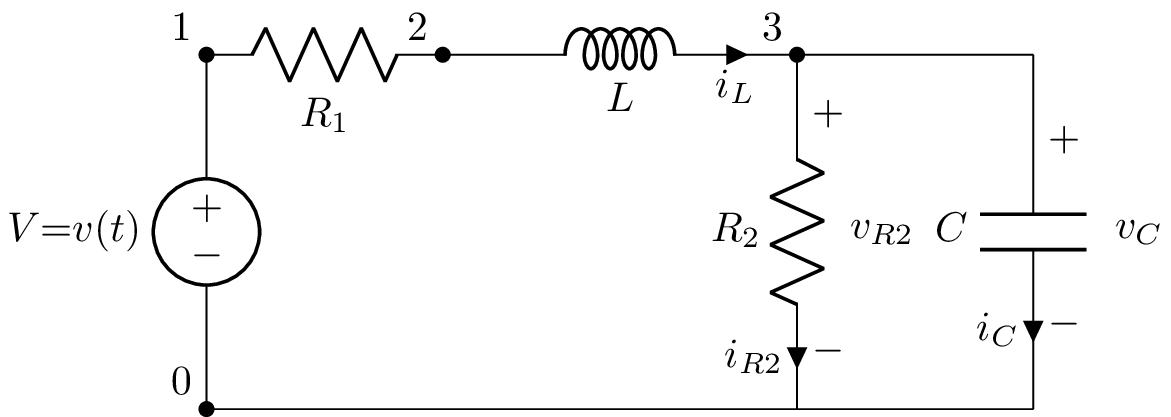
This circuit has two reactive components and thus there are two state variables; the current through L and the voltage across C.
The state equations are shown using the state_equations() method:
>>> ss.state_equations()
⎡d         ⎤   ⎡-R₁  -1  ⎤
⎢──(i_L(t))⎥   ⎢───  ─── ⎥            ⎡1⎤
⎢dt        ⎥   ⎢ L    L  ⎥ ⎡i_L(t)⎤   ⎢─⎥
⎢          ⎥ = ⎢         ⎥⋅⎢      ⎥ + ⎢L⎥⋅[v(t)]
⎢d         ⎥   ⎢-1   -1  ⎥ ⎣v_C(t)⎦   ⎢ ⎥
⎢──(v_C(t))⎥   ⎢───  ────⎥            ⎣0⎦
⎣dt        ⎦   ⎣ C   C⋅R₂⎦
The output equations are shown using the output_equations() method:
>>> ss.output_equations()
⎡v₁(t)⎤   ⎡0    0⎤            ⎡1⎤
⎢     ⎥   ⎢      ⎥ ⎡i_L(t)⎤   ⎢ ⎥
⎢v₂(t)⎥ = ⎢-R₁  0⎥⋅⎢      ⎥ + ⎢1⎥⋅[v(t)]
⎢     ⎥   ⎢      ⎥ ⎣v_C(t)⎦   ⎢ ⎥
⎣v₃(t)⎦   ⎣0    1⎦            ⎣0⎦
For further details see State-space analysis.
Other circuit methods
Isc(Np, Nm) Short-circuit current between nodes Np and Nm.
Voc(Np, Nm) Open-circuit voltage between nodes Np and Nm.
isc(Np, Nm) Short-circuit t-domain current between nodes Np and Nm.
voc(Np, Nm) Open-circuit t-domain voltage between nodes Np and Nm.
admittance(Np, Nm) s-domain admittance between nodes Np and Nm.
impedance(Np, Nm) s-domain impedance between nodes Np and Nm.
kill() Remove independent sources.
kill_except(sources) Remove independent sources except ones specified.
transfer(N1p, N1m, N2p, N2m) Voltage transfer function V2/V1, where V1 = V[N1p] - V[N1m], V2 = V[N2p] - V[N2m].
thevenin(Np, Nm) Thevenin model between nodes Np and Nm.
norton(Np, Nm) Norton model between nodes Np and Nm.
twoport(self, N1p, N1m, N2p, N2m) Create two-port component where I1 is the current flowing into N1p and out of N1m, I2 is the current flowing into N2p and out of N2m, V1 = V[N1p] - V[N1m], V2 = V[N2p] - V[N2m].
add(component) Add component from net list.
remove(component) Remove component from net list.
netfile_add(filename) Add netlist from file.
s_model() Convert circuit to s-domain model.
pre_initial_model() Convert circuit to pre-initial model.
ac() Create netlist for AC components of independent sources.
dc() Create netlist for DC components of independent sources.
transient() Create netlist for transient components of independent sources.
laplace() Create netlist with Laplace representations of independent source values.
Plotting
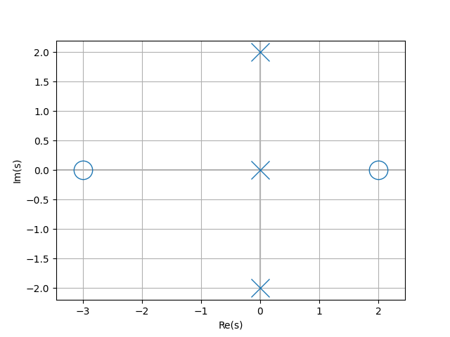
Lcapy expressions have a plot() method; this differs depending on the domain (see Plotting). For example, the plot() method for Laplace-domain expressions produces a pole-zero plot. Here’s an example:
from lcapy import s, j, transfer
from matplotlib.pyplot import savefig

H = transfer((s - 2) * (s + 3) / (s * (s - 2 * j) * (s + 2 * j)))
H.plot()

savefig('tf1-pole-zero-plot.png')
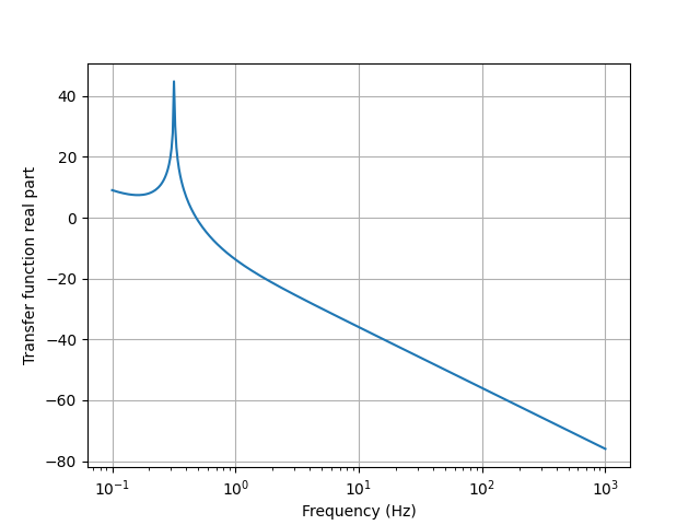
The plot() method for f-domain and \(\omega\)-domain expressions produce spectral plots, for example,
from lcapy import s, j, pi, f, transfer, j2pif
from matplotlib.pyplot import savefig
from numpy import logspace

# Note, this has a marginally stable impulse response since it has a
# pole at s = 0.
H = transfer((s - 2) * (s + 3) / (s * (s - 2 * j) * (s + 2 * j)))

fv = logspace(-1, 3, 400)
H(j2pif).dB.plot(fv, log_scale=True)

savefig('tf1-bode-plot.png')
Schematics
Schematics can be generated from a netlist and from one-port networks. In both cases the drawing is performed using the LaTeX Circuitikz package. The schematic can be displayed interactively or saved to a pdf, png, or pgf file.
Netlist schematics
Hints are required to designate component orientation and explicit wires are required to link nodes of the same potential but with different coordinates. For more details see Schematics.
Here’s an example:
>>> from lcapy import Circuit
>>> cct = Circuit("""
... V1 1 0 {V(s)}; down
... R1 1 2; right
... C1 2 0_2; down
... W1 0 0_2; right""")
>>> cct.draw('schematic.pdf')
Note, the orientation hints are appended to the netlist strings with a semicolon delimiter. The drawing direction is with respect to the first node. The component W1 is a wire. Nodes with an underscore in their name are not drawn with a closed blob.
Here’s another example, this time loading the netlist from a file:
>>> from lcapy import Circuit
>>> cct = Circuit('voltage-divider.sch')
>>> cct.draw('voltage-divider.pdf')
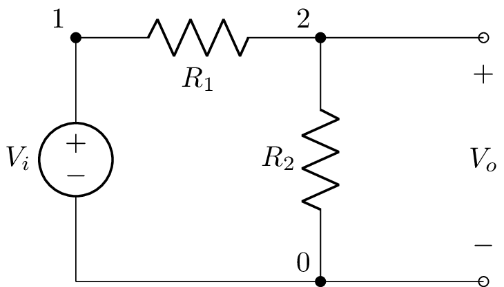
Here are the contents of the file ‘voltage-divider.sch’:
V1 1 0_1 dc V; down
R1 1 2 R1; right
R2 2 0 R2; down
P1 2_2 0_2; down
W1 2 2_2; right
W2 0_1 0; right
W3 0 0_2; right
Here, P1 defines a port. This is shown as a pair of open blobs.
Here’s the resulting schematic:
Many other components can be drawn than can be simulated. This includes non-linear devices such as transistors and diodes and time varying components such as switches. For example, here’s a common base amplifier,
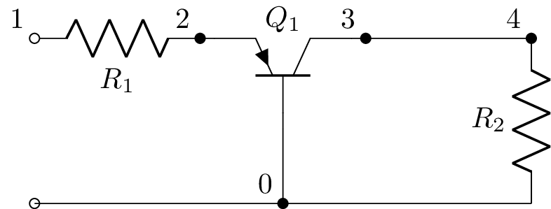
This is described by the netlist:
Q1 3 0 2 pnp; up
R1 1 2;right
R2 4 0_4;down
P1 1 0_1;down
W 0_1 0;right
W 0 0_4;right
W 3 4;right
Network schematics
One-port networks can be drawn with a horizontal layout. Here’s an example:
>>> from lcapy import R, C, L
>>> ((R(1) + L(2)) | C(3)).draw()
Here’s the result:

The s-domain model can be drawn using:
>>> from lcapy import R, C, L
>>> ((R(1) + L(2)) | C(3)).s_model().draw()
This produces:

Internally, Lcapy converts the network to a netlist and then draws the netlist. The netlist can be found using the netlist() method, for example:
>>> from lcapy import R, C, L
>>> print(((R(1) + L(2)) | C(3)).netlist())
yields:
W 1 3; right, size=0.5
W 3 4; up, size=0.4
W 3 5; down, size=0.4
W 6 2; right, size=0.5
W 6 7; up, size=0.4
W 6 8; down, size=0.4
R 4 9 1; right
W 9 10; right, size=0.5
L 10 7 2 0; right
C 5 8 3 0; right
Note, the components have anonymous identifiers.
Bells and whistles
Parameterization
Transfer functions (or any s-domain expression) can be parameterized with the parameterize() method (see Parameterization). This returns a tuple. The first element is the parameterized expression and the second element is a dictionary of substitutions.
Here’s a second order example:
>>> H2 = 3 / (s**2 + 2*s + 4)
>>> H2
     3
────────────
 2
s  + 2⋅s + 4
>>> H2p, defs = H2.parameterize()
>>> H2p
           K
───────────────────
  2               2
ω₀  + 2⋅ω₀⋅s⋅ζ + s

>>> defs
{K: 3, omega_0: 2, zeta: 1/2}
Network synthesis
Network synthesis creates a network from an impedance (or admittance), see Network synthesis.
Discrete-time signals
Lcapy supports discrete-time signals and provides z-transforms, discrete Fourier transforms (DFT), and discrete-time Fourier transforms (DTFT), see Discrete-time signals. The signals can be represented as expressions or sequences of symbolic elements. For example:
 >>> x = seq((1, 2, 3))
 {_1, 2, 3}
 >>> x.expr
 δ[n] + 3⋅δ[n - 2] + 2⋅δ[n - 1]
 >>> x.expr(z)
     2   3
 1 + ─ + ──
     z    2
         z

>>> H = (z + 2) / z**2
>>> H.difference_equation('x', 'y')
y(n) = 2⋅x(n - 2) + x(n - 1)
Jupyter (IPython) notebooks
Jupyter notebooks allow interactive markup of python code and text. A number of examples are provided in the lcapy/doc/examples/notebooks directory. Before these notebooks can be viewed in a browser you need to start a Jupyter notebook server.
$ cd lcapy/doc/examples/notebooks
$ jupyter notebook
Alternatively, they can be viewed online at https://github.com/mph-/lcapy/tree/master/doc/examples/notebooks.