Circuit analysis
Introduction
Lcapy can only analyse linear time invariant (LTI) circuits, this includes both passive and active circuits. Time invariance means that the circuit parameters cannot change with time; i.e., capacitors cannot change value with time. It also means that the circuit configuration cannot change with time, i.e., contain switches (although switching problems can be analysed, see Switching analysis).
Linearity means that superposition applies—if you double the voltage of a source, the current (anywhere in the circuit) due to that source will also double. This restriction rules out components such as diodes and transistors that have a non-linear relationship between current and voltage (except in circumstances where the relationship can be approximated as linear around some constant value—small signal analysis). Linearity also rules out capacitors where the capacitance varies with voltage and inductors with hysteresis.
Networks and netlists
Lcapy circuits can be created using a netlist specification (see Netlists) or by combinations of components (see Networks). For example, here are two ways to create the same circuit:
>>> cct1 = (Vstep(10) + R(1)) | C(2)
>>> cct2 = Circuit()
>>> cct2.add('V1 1 0 step 10')
>>> cct2.add('R1 1 2 1')
>>> cct2.add('C1 2 0 2')
The two approaches have many attributes and methods in common. For example,
>>> cct1.is_causal
True
>>> cct2.is_causal
True
>>> cct1.is_dc
False
>>> cct2.is_dc
False
However, there are subtle differences. For example,
>>> cct1.Voc.laplace()
   5
──────
 2   s
s  + ─
     2
>>> cct2.Voc(2, 0).laplace()
   5
──────
 2   s
s  + ─
     2
Notice, the second example requires specific nodes to determine the open-circuit voltage across. The advantage of the netlist approach is that component names can be used, for example,
>>> cct2.V1.V.laplace()
   5
──────
 2   s
s  + ─
     2
Linear circuit analysis
The voltages and currents in a circuit can be found by applying Kirchhoff’s current and voltage laws in conjunction with the relationships between voltage and current for resistors, capacitors, and inductors. However, this leads to a system of simultaneous integro-differential equations to solve. This is not fun!
If the system is linear, superposition can be applied to consider the effect of each independent current and voltage source in isolation and summing the results. Furthermore, differential equations are not required for DC signals and can be avoided by using transform techniques (phasor analysis for AC signals and Laplace analysis for transient signals). Thus for each domain, the voltages and currents can be found by solving a system of linear equations.
Lcapy’s algorithm for solving a circuit is:
If a capacitor or inductor is found to have initial conditions, then the circuit is analysed as an initial value problem using Laplace methods. In this case, the sources are ignored for \(t<0\) and the result is only known for \(t\ge 0\).
If there are no capacitors and inductors and if none of the independent sources are specified in the Laplace domain, then time-domain analysis is performed (since no derivatives or integrals are required).
Finally, Lcapy tries to decompose the sources into DC, AC, transient, and noise components. The circuit is analysed for each source category using the appropriate transform domain (phasors for AC, Laplace domain for transients) and the results are added. If there are multiple noise sources, these are considered independently since they are assumed to be uncorrelated.
The method that Lcapy uses can be found using the describe() method. For example,
>>> cct = Circuit("""
... V1 1 0 {1 + u(t)}
... R1 1 2
... L1 2 0""")
>>> cct.describe()
This is solved using superposition.
DC analysis is used for source V1.
Laplace analysis is used for source V1.
>>> cct = Circuit("""
... V1 1 0 {1 + u(t)}
... R1 1 2
... V2 2 0 ac""")
>>> cct.describe()
This is solved using superposition.
Time-domain analysis is used for source V1.
Phasor analysis is used for source V2.
DC analysis
The simplest special case is for a DC independent source. DC is an idealised concept—it impossible to generate—but is a good approximation for very slowly changing sources. With a DC independent source the dependent sources are also DC and thus no voltages or currents change. Thus capacitors can be replaced with open-circuits and inductors can be replaced with short-circuits. Note, Lcapy places a conductance in parallel with each capacitor and considers the limit as the conductance goes to zero.
AC (phasor) analysis
AC, like DC, is an idealised concept. It allows circuits to be analysed using phasors and impedances. The use of impedances avoids solving integro-differential equations in the time domain.
Transient (Laplace) analysis
The response due to a transient excitation from an independent source can be analysed using Laplace analysis. Since the unilateral transform is not unique (it ignores the circuit behaviour for \(t < 0\)), the response can only be determined for \(t \ge 0\).
If the independent sources are known to be causal (a causal signal is zero for \(t < 0\) analogous to a causal impulse response) and the initial conditions (i.e., the voltages across capacitors and currents through inductors) are zero, then the response is 0 for \(t < 0\). Thus in this case, the response can be specified for all \(t\).
The response due to a general non-causal excitation is hard to determine using Laplace analysis. One strategy is to use circuit analysis techniques to determine the response for \(t < 0\), compute the pre-initial conditions, and then use Laplace analysis to determine the response for \(t \ge 0\). Note, the pre-initial conditions at \(t = 0_{-}\) are required. These differ from the initial conditions at \(t = 0\) whenever a Dirac delta (or its derivative) excitation is considered. Determining the initial conditions is not straightforward for arbitrary excitations and at the moment Lcapy expects you to do this!
The use of pre-initial conditions also allows switching circuits to be considered (see Switching analysis). In this case the independent sources are ignored for \(t < 0\) and the result is only known for \(t \ge 0\).
Note if any of the pre-initial conditions are non-zero and the independent sources are causal then either we have an initial value problem or a mistake has been made. Lcapy assumes that if any of the inductors and capacitors have explicit initial conditions, then the circuit is to be analysed as an initial value problem with the independent sources ignored for \(t \ge 0\). In this case a DC source is not DC since it is considered to switch on at \(t = 0\).
Switching analysis
Whenever a circuit has a switch it is time variant. The opening or closing of the switch changes the circuit and can produce transients. Be careful with switching circuits since it easy to produce a circuit that cannot be analysed; for example, an inductor may be open-circuited when a switch opens.
Lcapy can solve circuits with switches by converting them to an initial value problem (IVP) with the convert_IVP() method. This has a time argument that is used to determine the states of the switches. The circuit is solved prior to the moment when the last switch activates and this is used to provide initial values for the moment when the last switch activates. If there are multiple switches with different activation times, the initial values are evaluated recursively. See Switching circuits for some examples.
Noise analysis
Each noise source is assigned a noise identifier (nid), see Noise signals. Noise expressions with different nids are assumed to be independent and thus represent different noise realisations.
Lcapy analyses the circuit for each noise realisation independently and stores the result for each realisation separately. For example,
>>> a = Circuit()
>>> a.add('Vn1 1 0 noise 3')
>>> a.add('Vn2 2 1 noise 4')
>>> a[2].V
{n1: 3, n2: 4}
>>> a[1].V
{n1: 3}
>>> a[2].V - a[1].V
{n1: 0, n2: 4}
>>> a[2].V.n
5
Notice that the .n attribute returns the total noise found by adding each noise component in quadrature, i.e., \(\sqrt{3^2 + 4^2},\) since the noise components have different nids and are thus independent.
Each resistor in a circuit can be converted into a series combination of an ideal resistor and a noise voltage source using the noise_model method.
Mesh analysis
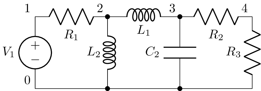
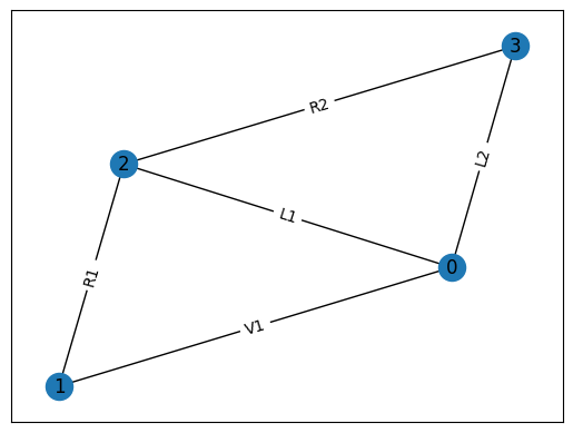
Lcapy can output the mesh equations for a planar circuit by applying Kirchhoff’s voltage law around each loop in the circuit. For example, consider the netlist:
>>> cct = Circuit("""
...V1 1 0; down
...R1 1 2; right
...L1 2 3; right
...R2 3 4; right
...L2 2 0_2; down
...C2 3 0_3; down
...R3 4 0_4; down
...W 0 0_2; right
...W 0_2 0_3; right
...W 0_3 0_4; right""")
>>> cct.draw()
The mesh equations are found using:
>>> l = cct.mesh_analysis()
>>> l.mesh_equations()
⎧                                              t
⎪                                              ⌠
⎪                                              ⎮  (-i₁(τ) + i₃(τ)) dτ
⎨                                              ⌡
⎪          d               d                   -∞
⎪i₁(t): L₁⋅──(-i₁(t)) + L₂⋅──(i₁(t) - i₂(t)) + ────────────────────── = 0,
⎩          dt              dt                            C₂
           d
 i₂(t): L₂⋅──(i₁(t) - i₂(t)) - R₁⋅i₂(t) + v₁(t) = 0,
           dt
                                t
                               ⌠                         ⎪
                               ⎮  (-i₁(τ) + i₃(τ)) dτ    ⎪
                               ⌡                         ⎬
                               -∞                        ⎪
 i₃(t): -R₂⋅i₃(t) - R₃⋅i₃(t) + ────────────────────── = 0⎪
                                   C₂                    ⎭
Note, the dictionary is keyed by the mesh current.
The mesh equations can be formulated in the s-domain using:
>>> l = cct.laplace().mesh_analysis()
>>> l.mesh_equations()
⎧                              I₁(s) - I₂(s)                                                  I₁(s) - I₂(s)                                               1    ⎫
⎨I₁(s): -R₂⋅I₁(s) - R₃⋅I₁(s) + ───────────── = 0, I₂(s): -L₁⋅s⋅I₂(s) + L₂⋅s⋅(I₂(s) - I₃(s)) + ───────────── = 0, I₃(s): L₂⋅s⋅(I₂(s) - I₃(s)) - R₁⋅I₃(s) + ─ = 0⎬
⎩                                   C₂⋅s                                                           C₂⋅s                                                   s    ⎭
The system of equations can be formulated in matrix form as \(\mathbf{A} \mathbf{y} = \mathbf{b}\) using:
>>> l.matrix_equations(form='A y = b')
⎡      R₁                                     ⎤
⎢-L₂ - ──          0                 L₂       ⎥
⎢      s                                      ⎥
⎢                                             ⎥        ⎡-1 ⎤
⎢            R₂   R₃     1          -1        ⎥ ⎡I₁⎤   ⎢───⎥
⎢   0      - ── - ── + ─────       ─────      ⎥ ⎢  ⎥   ⎢ s ⎥
⎢            s    s        2           2      ⎥⋅⎢I₂⎥ = ⎢   ⎥
⎢                      C₂⋅s        C₂⋅s       ⎥ ⎢  ⎥   ⎢ 0 ⎥
⎢                                             ⎥ ⎣I₃⎦   ⎢   ⎥
⎢                  1                       1  ⎥        ⎣ 0 ⎦
⎢  -L₂           ─────        -L₁ + L₂ - ─────⎥
⎢                    2                       2⎥
⎣                C₂⋅s                    C₂⋅s ⎦
The system of equations can be shown in a number of forms: y = Ainv b, Ainv b = y, A y = b, and b = A y. The inverse argument calculates the inverse of the A matrix.
The matrix is returned by the A attribute, the vector of unknowns by the y attribute, and the result vector by the b attribute.
The mesh currents can be found with the solve_laplace() method. This solves the circuit using Laplace transform methods and returns a dictionary of results.
The mesh analysis implementation does not support twoport components, such as transformers and gyrators.
Nodal analysis
Lcapy can output the nodal equations by applying Kirchhoff’s current law at each node in a circuit. For example, consider the netlist:
>>> cct = Circuit("""
...V1 1 0 {u(t)}; down
...R1 1 2; right
...L1 2 3; right
...R2 3 4; right
...L2 2 0_2; down
...C2 3 0_3; down
...R3 4 0_4; down
...W 0 0_2; right
...W 0_2 0_3; right
...W 0_3 0_4; right""")
>>> cct.draw()
The nodal equations are found using:
>>> n = cct.nodal_analysis()
>>> n.nodal_equations()
⎧
⎪
⎪
⎨
⎪
⎪ 1: v₁(t) = u(t),
⎩
                          t              t
                         ⌠              ⌠
                         ⎮  v₂(τ) dτ    ⎮  (v₂(τ) - v₃(τ)) dτ
                         ⌡              ⌡
      -v₁(t) + v₂(t)   -∞             -∞
  2: ──────────────── + ──────────── + ─────────────────────── = 0,
             R₁               L₂                   L₁

                                        t
                                       ⌠
                                       ⎮  (-v₂(τ) + v₃(τ)) dτ
                                       ⌡
        d            v₃(t) - v₄(t)   -∞
  3: C₂⋅──(v₃(t)) + ─────────────── + ──────────────────────── = 0,
        dt                  R₂                  L₁

                                   ⎫
                                   ⎪
                                   ⎪
                                   ⎬
      v₄(t)   -v₃(t) + v₄(t)       ⎪
  4: ────── + ──────────────── = 0 ⎪
       R₃            R₂            ⎭
Note, these are keyed by the node names. The node_prefix argument can be used with nodal_analysis() to resolve ambiguities with component voltages and node voltages.
The nodal equations can be formulated in the s-domain using:
>>> na = cct.laplace().nodal_analysis()
>>> na.nodal_equations()
⎧           1
⎨1: V₁(s) = ─,
⎩           s
    -V₁(s) + V₂(s)   V₂(s)   V₂(s) - V₃(s)
 2: ────────────── + ───── + ───────────── = 0,
          R₁          L₂⋅s        L₁⋅s
                 V₃(s) - V₄(s)   -V₂(s) + V₃(s)
 3: C₂⋅s⋅V₃(s) + ───────────── + ────────────── = 0,
                       R₂             L₁⋅s
    V₄(s)   -V₃(s) + V₄(s)    ⎫
 4: ───── + ────────────── = 0⎬
      R₃          R₂          ⎭
The system of equations can be formulated in matrix form as \(\mathbf{A} \mathbf{y} = \mathbf{b}\) using:
>>> l.matrix_equations(form='A y = b')
⎡ 1             0                    0               0     ⎤
⎢                                                          ⎥
⎢-1     1       1       1           -1                     ⎥
⎢────  ──── + ───── + ─────        ─────             0     ⎥        ⎡1⎤
⎢R₁⋅s  R₁⋅s       2       2            2                   ⎥ ⎡V₁⎤   ⎢─⎥
⎢             L₂⋅s    L₁⋅s         L₁⋅s                    ⎥ ⎢  ⎥   ⎢s⎥
⎢                                                          ⎥ ⎢V₂⎥   ⎢ ⎥
⎢              -1                  1       1       -1      ⎥⋅⎢  ⎥ = ⎢0⎥
⎢ 0           ─────          C₂ + ──── + ─────     ────    ⎥ ⎢V₃⎥   ⎢ ⎥
⎢                 2               R₂⋅s       2     R₂⋅s    ⎥ ⎢  ⎥   ⎢0⎥
⎢             L₁⋅s                       L₁⋅s              ⎥ ⎣V₄⎦   ⎢ ⎥
⎢                                                          ⎥        ⎣0⎦
⎢                                  -1            1      1  ⎥
⎢ 0             0                  ────         ──── + ────⎥
⎣                                  R₂⋅s         R₃⋅s   R₂⋅s⎦
The system of equations can be shown in a number of forms: y = Ainv b, Ainv b = y, A y = b, and b = A y. The invert argument calculates the inverse of the A matrix (see System of equations).
The matrix is returned by the A attribute, the vector of unknowns by the y attribute, and the result vector by the b attribute.
The node voltages can be found with the solve_laplace() method. This solves the circuit using Laplace transform methods and returns a dictionary of results.
The nodal analysis implementation does not support twoport components, such as transformers and gyrators. Instead use modified nodal analysis.
Modified nodal analysis
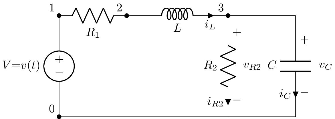
Here’s an example with an independent source (V1) that has a DC component and an unknown component that is considered a transient:
>>> from lcapy import Circuit
>>> a = Circuit("""
... V1 1 0 {10 + v(t)}; down
... R1 1 2; right
... L1 2 3; right=1.5, i={i_L}
... R2 3 0_3; down=1.5, i={i_{R2}}, v={v_{R2}}
... W 0 0_3; right
... W 3 3_a; right
... C1 3_a 0_4; down, i={i_C}, v={v_C}
... W 0_3 0_4; right""")
The corresponding circuit for DC analysis can be found using the dc() method:
>>> a.dc()
V1 1 0 dc {10}; down
R1 1 2; right
L1 2 3 L1; right=1.5, i={i_L}
R2 3 0_3; i={i_{R2}}, down=1.5, v={v_{R2}}
W 0 0_3; right
W 3 3_a; right
C1 3_a 0_4 C1; i={i_C}, down, v={v_C}
W 0_3 0_4; right
The equations used to solve this can be found with the matrix_equations() method:
>>> ac.dc().matrix_equations()
                                -1
         ⎛⎡1    -1            ⎤⎞
         ⎜⎢──   ───  0   1  0 ⎥⎟
         ⎜⎢R₁    R₁           ⎥⎟
⎡V₁  ⎤   ⎜⎢                   ⎥⎟   ⎡0 ⎤
⎢    ⎥   ⎜⎢-1   1             ⎥⎟   ⎢  ⎥
⎢V₂  ⎥   ⎜⎢───  ──   0   0  1 ⎥⎟   ⎢0 ⎥
⎢    ⎥   ⎜⎢ R₁  R₁            ⎥⎟   ⎢  ⎥
⎢V₃  ⎥ = ⎜⎢                   ⎥⎟  ⋅⎢0 ⎥
⎢    ⎥   ⎜⎢          1        ⎥⎟   ⎢  ⎥
⎢I_V1⎥   ⎜⎢ 0    0   ──  0  -1⎥⎟   ⎢10⎥
⎢    ⎥   ⎜⎢          R₂       ⎥⎟   ⎢  ⎥
⎣I_L1⎦   ⎜⎢                   ⎥⎟   ⎣0 ⎦
         ⎜⎢ 1    0   0   0  0 ⎥⎟
         ⎜⎢                   ⎥⎟
         ⎝⎣ 0    1   -1  0  0 ⎦⎠
Here V1, V2, and V3 are the unknown node voltages for nodes 1, 2, and 3. I_V1 is the current through V1 and I_L1 is the current through L1.
The equations are similar for the transient response:
>>> a.transient().matrix_equations()
                                             -1
            ⎛⎡1    -1                      ⎤⎞
            ⎜⎢──   ───      0      1    0  ⎥⎟
            ⎜⎢R₁    R₁                     ⎥⎟
⎡V₁(s)  ⎤   ⎜⎢                             ⎥⎟   ⎡ 0  ⎤
⎢       ⎥   ⎜⎢-1   1                       ⎥⎟   ⎢    ⎥
⎢V₂(s)  ⎥   ⎜⎢───  ──       0      0    1  ⎥⎟   ⎢ 0  ⎥
⎢       ⎥   ⎜⎢ R₁  R₁                      ⎥⎟   ⎢    ⎥
⎢V₃(s)  ⎥ = ⎜⎢                             ⎥⎟  ⋅⎢ 0  ⎥
⎢       ⎥   ⎜⎢                 1           ⎥⎟   ⎢    ⎥
⎢I_V1(s)⎥   ⎜⎢ 0    0   C₁⋅s + ──  0   -1  ⎥⎟   ⎢V(s)⎥
⎢       ⎥   ⎜⎢                 R₂          ⎥⎟   ⎢    ⎥
⎣I_L1(s)⎦   ⎜⎢                             ⎥⎟   ⎣ 0  ⎦
            ⎜⎢ 1    0       0      0    0  ⎥⎟
            ⎜⎢                             ⎥⎟
            ⎝⎣ 0    1      -1      0  -L₁⋅s⎦⎠
See System of equations for formatting of the equations.
State-space analysis
Lcapy can generate a state-space representation of a circuit. It chooses the currents through inductors and the voltage across capacitors as the state variables. It can then generate the state and output equations as well as the characteristic polynomial, etc.
However, Lcapy does not support degenerate circuits (see Degenerate circuits). These are circuits with a loop consisting only of voltage sources and/or capacitors, or a cut set consisting only of current sources and/or inductors. Using simplify() on the netlist can resolve some of these problems.
State-space analysis is performed by accessing the ss attribute of a circuit (this generates a StateSpace object and caches the result), e.g.,
>>> from lcapy import Circuit
>>> a = Circuit("""
... V 1 0 {v(t)}; down
... R1 1 2; right
... L 2 3; right=1.5, i=i_L
... R2 3 0_3; down=1.5, i=i_{R2}, v=v_{R2}
... W 0 0_3; right
... W 3 3_a; right
... C 3_a 0_4; down, i=i_C, v=v_C
... W 0_3 0_4; right""")
>>> ss = a.ss
If you want to control which node voltages or branch currents are used as output variables, use the state_space() method.
This circuit has two reactive components and thus there are two state variables; the current through L and the voltage across C.
The state variable vector is shown using the x attribute:
>>> ss.x
⎡i_L(t)⎤
⎢      ⎥
⎣v_C(t)⎦
The initial values of the state variable vector are shown using the x0 attribute:
>>> ss.x0
⎡0⎤
⎢ ⎥
⎣0⎦
The independent source vector is shown using the u attribute. In this example, there is a single independent source:
>>> ss.u
[v(t)]
The output vector can either be the nodal voltages, the branch currents, or both. By default the nodal voltages are chosen. This vector is shown using the y attribute:
>>> ss.y
⎡v₁(t)⎤
⎢     ⎥
⎢v₂(t)⎥
⎢     ⎥
⎣v₃(t)⎦
The state equations are shown using the state_equations() method:
>>> ss.state_equations()
⎡d         ⎤   ⎡-R₁  -1  ⎤
⎢──(i_L(t))⎥   ⎢───  ─── ⎥            ⎡1⎤
⎢dt        ⎥   ⎢ L    L  ⎥ ⎡i_L(t)⎤   ⎢─⎥
⎢          ⎥ = ⎢         ⎥⋅⎢      ⎥ + ⎢L⎥⋅[v(t)]
⎢d         ⎥   ⎢-1   -1  ⎥ ⎣v_C(t)⎦   ⎢ ⎥
⎢──(v_C(t))⎥   ⎢───  ────⎥            ⎣0⎦
⎣dt        ⎦   ⎣ C   C⋅R₂⎦
The output equations are shown using the output_equations() method:
>>> ss.output_equations()
⎡v₁(t)⎤   ⎡0    0⎤            ⎡1⎤
⎢     ⎥   ⎢      ⎥ ⎡i_L(t)⎤   ⎢ ⎥
⎢v₂(t)⎥ = ⎢-R₁  0⎥⋅⎢      ⎥ + ⎢1⎥⋅[v(t)]
⎢     ⎥   ⎢      ⎥ ⎣v_C(t)⎦   ⎢ ⎥
⎣v₃(t)⎦   ⎣0    1⎦            ⎣0⎦
The A, B, C, and D matrices are obtained using the attributes of the same name. For example,
>>> ss.A
⎡-R₁   -1  ⎤
⎢───   ─── ⎥
⎢ L     L  ⎥
⎢          ⎥
⎢ 1    -1  ⎥
⎢───   ────⎥
⎣ C    C⋅R₂⎦
>>> ss.B
⎡1⎤
⎢─⎥
⎢L⎥
⎢ ⎥
⎣0⎦
>>> ss.C
⎡0    0⎤
⎢      ⎥
⎢-R₁  0⎥
⎢      ⎥
⎣0    1⎦
>>> ss.D
⎡1⎤
⎢ ⎥
⎢1⎥
⎢ ⎥
⎣0⎦
The Laplace transforms of the state variable vector, the independent source vector, and the output vector are accessed using the X, U, and Y attributes. For example,
>>> ss.X
⎡I_L(s)⎤
⎢      ⎥
⎣V_C(s)⎦
The s-domain state-transition matrix is given by the Phi attribute and the time-domain state-transition matrix is given by the phi attribute. For example,
>>> ss.Phi
⎡                  1                                                   ⎤
⎢             s + ────                                                 ⎥
⎢                 C⋅R₂                              -1                 ⎥
⎢  ──────────────────────────────    ──────────────────────────────────⎥
⎢   2   s⋅(C⋅R₁⋅R₂ + L)   R₁ + R₂      ⎛ 2   s⋅(C⋅R₁⋅R₂ + L)   R₁ + R₂⎞⎥
⎢  s  + ─────────────── + ───────    L⋅⎜s  + ─────────────── + ───────⎟⎥
⎢            C⋅L⋅R₂        C⋅L⋅R₂      ⎝          C⋅L⋅R₂        C⋅L⋅R₂⎠⎥
⎢                                                                      ⎥
⎢                                                      R₁              ⎥
⎢                                                  s + ──              ⎥
⎢                1                                     L               ⎥
⎢──────────────────────────────────    ──────────────────────────────  ⎥
⎢  ⎛ 2   s⋅(C⋅R₁⋅R₂ + L)   R₁ + R₂⎞     2   s⋅(C⋅R₁⋅R₂ + L)   R₁ + R₂  ⎥
⎢C⋅⎜s  + ─────────────── + ───────⎟    s  + ─────────────── + ───────  ⎥
⎣  ⎝          C⋅L⋅R₂        C⋅L⋅R₂⎠              C⋅L⋅R₂        C⋅L⋅R₂  ⎦
The system transfer functions are given by the G attribute and the impulse responses are given by the g attributes, for example:
>>> ss.G
⎡                 1                  ⎤
⎢                                    ⎥
⎢           2    s      1            ⎥
⎢          s  + ──── + ───           ⎥
⎢               C⋅R₂   C⋅L           ⎥
⎢   ──────────────────────────────   ⎥
⎢    2   s⋅(C⋅R₁⋅R₂ + L)   R₁ + R₂   ⎥
⎢   s  + ─────────────── + ───────   ⎥
⎢             C⋅L⋅R₂        C⋅L⋅R₂   ⎥
⎢                                    ⎥
⎢                 1                  ⎥
⎢────────────────────────────────────⎥
⎢    ⎛ 2   s⋅(C⋅R₁⋅R₂ + L)   R₁ + R₂⎞⎥
⎢C⋅L⋅⎜s  + ─────────────── + ───────⎟⎥
⎣    ⎝          C⋅L⋅R₂        C⋅L⋅R₂⎠⎦
The characteristic polynomial (system polynomial) is given by the P attribute, for example,
>>> ss.P
 2   s⋅(C⋅R₁⋅R₂ + L)   R₁ + R₂
s  + ─────────────── + ────────
          C⋅L⋅R₂        C⋅L⋅R₂
The roots of this polynomial are the eigenvalues of the system. These are given by the eigenvalues attribute. The corresponding eigenvectors are the columns of the modal matrix given by the M attribute. A diagonal matrix of the eigenvalues is returned by the Lambda attribute.
The singular values of the system are returned by the singular_values attribute.
For other methods and attributes, see Continuous-time state-space representation.
Degenerate circuits
Lcapy’s state-space analysis currently does not support degenerate circuits. These are circuits with a loop consisting only of voltage sources and/or capacitors, or a cut set consisting only of current sources and/or inductors. In these cases, choosing capacitor voltages (or inductor currents) for the state variables produces dependent state variables.
Consider an opamp integrator.
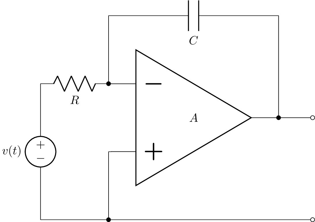
In this circuit, there is one state variable; the voltage across the capacitor. However, if the resistor was replaced with a wire, the voltage across the capacitor is constrained and so the capacitor voltage is not a state variable. Lcapy will produce the following error:
>>> Circuit('degenerate.sch').ss
ValueError: State-space analysis failed.
The MNA A matrix is not invertible for time analysis:
    Check voltage source is not short-circuited.
    Check for loop of voltage sources.
    Check for a loop consisting of voltage sources and/or capacitors.
A similar problem will occur if a capacitor is connected in parallel with the resistor. In this case, there is a loop consisting of voltage sources and capacitors (the output of the opamp is a voltage controlled voltage source). Thus both the capacitor voltages cannot be chosen as state variables since they are not independent (the voltage across one capacitor is constrained by the voltage across the other capacitor).
CircuitGraph
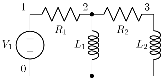
Both NodalAnalysis and LoopAnalysis use CircuitGraph to represent a netlist as a graph. This can be interrogated to find loops, etc. For example, consider the netlist:
>>> cct = Circuit("""
...V1 1 0; down
...R1 1 2; right
...L1 2 0_2; down
...R2 1 3; right
...L2 3 0_3; down
...W 0 0_2; right
...W 0_2 0_3; right""")
>>> cct.draw()
The graph is:
The loops in the graph can be found using:
>>> cg = cct.circuit_graph()
>>> cg.loops()
[['0', '1', '3'], ['0', '1', '2']]
>>> cg.draw()
Here’s another example:
>>> cct = Circuit("""
...V1 1 0; down
...R1 1 2; right
...L1 2 3; right
...R2 3 4; right
...L2 2 0_2; down
...C2 3 0_3; down
...R3 4 0_4; down
...W 0 0_2; right
...W 0_2 0_3; right
...W 0_3 0_4; right""")
>>> cct.draw()
The graph is:
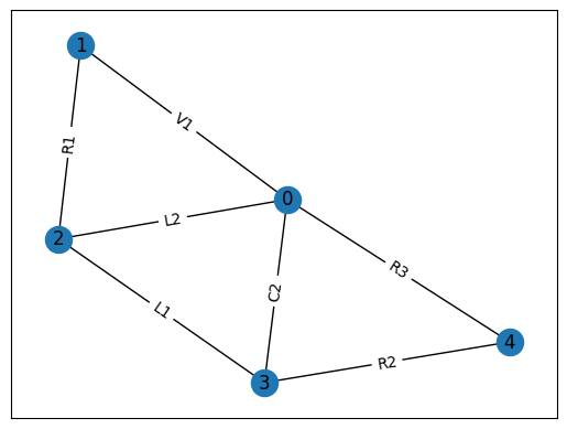
The loops in the graph can be found using:
>>> cg = cct.circuit_graph()
 >>> cg.loops()
 [['0', '3', '4'], ['0', '2', '3'], ['0', '1', '2']]
 >>> cg.draw()
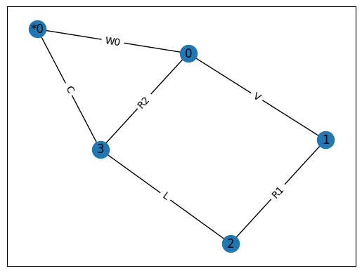
Note, circuit_graph() inserts dummy nodes and wires to avoid parallel edges. For example:
  >>> cct = Circuit("""
  V 1 0 {v(t)}; down
  R1 1 2; right
  L 2 3; right=1.5, i={i_L}
  R2 3 0_3; down=1.5, i={i_{R2}}, v={v_{R2}}
  W 0 0_3; right
  W 3 3_a; right
  C 3_a 0_4; down, i={i_C}, v={v_C}
  W 0_3 0_4; right""")
>>> cct.draw()

In this circuit, R2 is in parallel with C so Lcapy adds a dummy node 0* and a dummy component W01. The resulting graph is:
The cycle matrix for this example is:
>>> cct.cg.cycle_matrix
⎡-1  1  1  1   0⎤
⎢               ⎥
⎣0   0  0  -1  1⎦
where:
>>> cct.cg.cycle_matrix * cct.cg.branch_voltage_name_vector
⎡V_L + V_R1 + V_R2 - V_V⎤
⎢                       ⎥
⎣      V_C - V_R2       ⎦
This vector equates to zero. It is equivalent to Kirchhoff’s voltage law applied around all the loops.
The incidence matrix for this example is:
>>> cct.cg.incidence_matrix
⎡0   -1  0   -1  -1⎤
⎢                  ⎥
⎢1   0   -1  0   0 ⎥
⎢                  ⎥
⎢0   1   1   0   0 ⎥
⎢                  ⎥
⎣-1  0   0   1   1 ⎦
where:
>>> cct.cg.incidence_matrix * cct.cg.branch_current_name_vector
⎡-I_L - I_R2 - I_V⎤
⎢                 ⎥
⎢    I_C - I_R    ⎥
⎢                 ⎥
⎢    I_R + I_V    ⎥
⎢                 ⎥
⎣-I_C + I_L + I_R2⎦
This vector equates to zero. It is equivalent to Kirchhoff’s current law applied at all the nodes.
CircuitGraph attributes
DG the underlying directed networkx graph
UG the underlying undirected networkx graph
is_connected True if all the components are connected as a single graph
is_planar True if the component graph is planar
components list of component names
nodes the nodes comprising the graph
num_nodes the number of nodes comprising the graph
num_branches the number of branches (edges) comprising the graph
num_parts the number of separate graphs
nullity the number of meshes for a planar graph
rank the required number of node voltages for nodal analysis
node_connectivity the minimum connectivity of the graph. If 0, one or more components are connected, if 1, one or more components are connected at a single node, etc.
branch_name_list list of branches by component name
branch_current_name_vector branch current name vector. The branch current names are of the form I_cptname where cptname is the component name.
branch_voltage_name_vector branch voltage name vector. The branch voltage names are of the form V_cptname where cptname is the component name.
incidence_matrix the incidence matrix A. The number of rows is the number of nodes and the number of columns is the number of branches (edges). Each element is either 0, 1, or -1.
If I is a vector of edge currents then A I = 0.
cycle_matrix the cycle matrix B. The number of rows is the number of loops and the number of columns is the number of branches (edges). Each element is either 0, 1, or -1.
If V is a vector of branch voltages then B V = 0.
CircuitGraph methods
connected(node) set of components connected to node
cut_sets() list of cut sets, where each cut set is specified by a set of nodes
cut_vertices() list of cut vertices, where each cut vertex is a node
cut_edges() list of cut edges, where each cut edge is a tuple of nodes
loops() list of nodes where each loop is a list of nodes
loops_by_cpt_name() list of loops where each loop is a list of component names
draw(filename) draw the graph and save as filename. If filename is not specified, the graph is displayed.
node_edges(node) edges connected to specified node
component(node1, node2) component connected between specified nodes
in_series(cpt_name) set of component names in series with specified cpt_name
in_parallel(cpt_name) set of component names in parallel with specified cpt_name
tree() the minimum spanning tree.
links() the edges removed from the graph when forming the minimum spanning tree
unreachable_nodes(node) a list of nodes that have no path to node
has_path(node1, node2) True if there is a path from node1 to node2
Numerical simulation
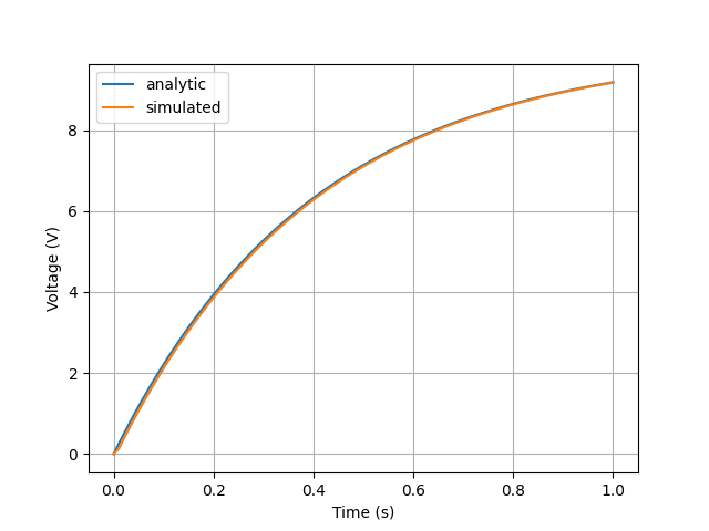
Lcapy can perform time-stepping numerical simulation of a circuit using numerical integration. Currently, only linear circuit elements can be simulated although this could be extended to non-linear components such as diodes and transistors. If you need to model a non-linear circuit numerically using Python, see PySpice (https://pypi.org/project/PySpice/).
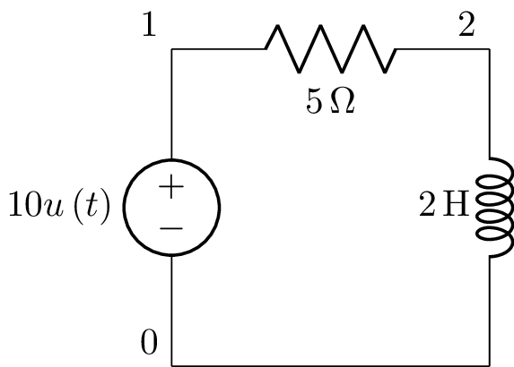
Here’s an example that compares the analytic and numerical results for an R-L circuit:
>>> from lcapy import Circuit
>>> from numpy import linspace
>>> from matplotlib.pyplot import savefig
>>>
>>> cct = Circuit("""
>>> V1 1 0 step 10; down
>>> R1 1 2 5; right
>>> L1 2 0_2 2; down
>>> W 0 0_2; right""")
>>>
>>> tv = linspace(0, 1, 100)
>>>
>>> results = cct.sim(tv)
>>>
>>> ax = cct.R1.v.plot(tv, label='analytic')
>>> ax.plot(tv, results.R1.v, label='simulated')
>>> ax.legend()
>>>
>>> savefig('sim1.png')
Integration methods
Currently the only supported numerical integration methods are trapezoidal and backward-Euler (others would be trivial to add). The trapezoidal method is the default since it is accurate but it can be unstable producing some oscillations. Unfortunately, there is no ideal numerical integration method and there is always a tradeoff between accuracy and stability.
Here’s an example of using the backward-Euler integration method:
>>> results = cct.sim(tv, integrator='backward-euler')
System of equations
A system of equations can be shown in a number of forms: y = Ainv b, Ainv b = y, A y = b, and b = A y. The invert argument calculates the inverse of the A matrix (see System of equations).